An Overview of RsNLME
rsnlme_overview.Rmd
The purpose of this vignette is to demonstrate how to utilize the
suite of R packages developed by Certara, specifically,
Certara.RsNLME, for a robust and reproducible
pharmacometric workflow using R. In the following examples, we will
demonstrate how to:
- Load the input dataset and visualize the data using
ggplot2. - Define the base model using
Certara.RsNLMEas well as mapping model variables to their corresponding input data columns. - Fit the base model.
- Import estimation results into R and create commonly used diagnostic
plots using
xposeandCertara.Xpose.NLME. - Accept parameter estimates from our base model execution, and create a new covariate model.
- Fit the covariate model and create covariate model diagnostic plots.
- Accept parameter estimates from the covariate model execution, and create a new VPC model.
- Fit the VPC model and create a binless and binned VPC using
tidyvpc. - Demonstrate functionality inside
Certara.ModelResultsandCertara.VPCResultsto facilitate code generation and reporting of model diagnostic plots, tables, and VPC.
Before we begin, a quick note about the differences between
S3 and S4 objects in R. Most objects
in R utilize the S3 class representation, and elements
inside the S3 class object can be accessed in R using the
$ operator. However, model objects in RsNLME
utilize the S4 class system. For S4 objects,
we access elements inside the class using the @ operator
(e.g., print(model@modelInfo@workingDir) to print the
directory of model output files).
For more details, see S4 versus S3.
Note: The following vignette was created with RsNLME v3.0.0. The
corresponding R script used in this example can be found in
RsNLME_Examples/TwoCptIVBolus_FitBaseModel_CovariateSearch_VPC_BootStrapping.R.
See RsNLME
Example Scripts.
Data
We will be using the built-in pkData from the
Certara.RsNLME package for the following examples.
pkData is a pharmacokinetic dataset containing 16 subjects
with single bolus dose.
pkData <- Certara.RsNLME::pkData

head(pkData)
#>   Subject Nom_Time Act_Time Amount Conc Age BodyWeight Gender
#> 1       1        0     0.00  25000 2010  22         73   male
#> 2       1        1     0.26     NA 1330  22         73   male
#> 3       1        1     1.10     NA  565  22         73   male
#> 4       1        2     2.10     NA  216  22         73   male
#> 5       1        4     4.13     NA  180  22         73   male
#> 6       1        8     8.17     NA  120  22         73   male
Exploratory Data Analysis (EDA)
Next, let’s perform some Exploratory Data Analysis (EDA) on our input
dataset by plotting drug concentration vs. time. Before calling our
ggplot2 code, we’ll convert the Subject column
to factor using mutate() from the
dplyr package, which will ensure the colors of the
Subject lines in our plot correctly display.
library(dplyr)
library(ggplot2)
library(magrittr)

pkData %>%
  mutate(Subject = as.factor(Subject)) %>%
  ggplot(aes(x = Act_Time, y = Conc, group = Subject, color = Subject)) +
   scale_y_log10() +
   geom_line() +
   geom_point() +
   ylab("Drug Concentration \n at the central compartment")
This plot suggests that a two-compartment model with IV bolus is a good starting point.
Build base model
We will use the pkmodel() function from the
Certara.RsNLME package to build our base two-compartment
model. Note that the modelName argument is used to create
the run folder for the associated output files from model execution.
library(Certara.RsNLME)

baseModel <- pkmodel(
  numCompartments = 2,
  data = pkData,
  ID = "Subject",
  Time = "Act_Time",
  A1 = "Amount",
  CObs = "Conc",
  modelName = "TwCpt_IVBolus_FOCE_ELS"
)
As demonstrated above, when we supply the data argument
to the pkmodel() function, we can directly map required
model variables to columns in the input data, supplying the associated
model variable names as additional arguments (e.g., ID,
Time, A1, CObs).
However, in some cases, we may not know what model variables require
column mappings given the different parameters specified in our model.
We can create our model without supplying column mappings inside the
pkmodel() function by adding the argument
columnMap = FALSE.
baseModel <-
  pkmodel(numCompartments = 2,
          columnMap = FALSE,
          modelName = "TwCpt_IVBolus_FOCE_ELS")
Next, we’ll specify the input dataset using the
dataMapping() function.
baseModel <- baseModel %>%
  dataMapping(pkData)
We can use the print() generic to view our model
information and required column mappings in the Column
Mappings section.
print(baseModel)
#>
#>  Model Overview
#>  -------------------------------------------
#> Model Name        :  TwCpt_IVBolus_FOCE_ELS
#> Working Directory :  /TestEnvironment/
#> Is population     :  TRUE
#> Model Type        :  PK
#>
#>  PK
#>  -------------------------------------------
#> Parameterization  :  Clearance
#> Absorption        :  Intravenous
#> Num Compartments  :  2
#> Dose Tlag?        :  FALSE
#> Elimination Comp ?:  FALSE
#> Infusion Allowed ?:  FALSE
#> Sequential        :  FALSE
#> Freeze PK         :  FALSE
#>
#>  PML
#>  -------------------------------------------
#> test(){
#>     cfMicro(A1,Cl/V, Cl2/V, Cl2/V2)
#>     dosepoint(A1)
#>     C = A1 / V
#>     error(CEps=0.1)
#>     observe(CObs=C * ( 1 + CEps))
#>     stparm(V = tvV * exp(nV))
#>     stparm(Cl = tvCl * exp(nCl))
#>     stparm(V2 = tvV2 * exp(nV2))
#>     stparm(Cl2 = tvCl2 * exp(nCl2))
#>     fixef( tvV = c(,1,))
#>     fixef( tvCl = c(,1,))
#>     fixef( tvV2 = c(,1,))
#>     fixef( tvCl2 = c(,1,))
#>     ranef(diag(nV,nCl,nV2,nCl2) =  c(1,1,1,1))
#> }
#>
#>  Structural Parameters
#>  -------------------------------------------
#>  V Cl V2 Cl2
#>  -------------------------------------------
#> Observations:
#> Observation Name :  CObs
#> Effect Name      :  C
#> Epsilon Name     :  CEps
#> Epsilon Type     :  Multiplicative
#> Epsilon frozen   :  FALSE
#> is BQL           :  FALSE
#>  -------------------------------------------
#>  Column Mappings
#>  -------------------------------------------
#> Model Variable Name : Data Column name
#> id                  : ?
#> time                : ?
#> A1                  : ?
#> CObs                : ?
Our baseModel object needs the following model variables
to be mapped to the corresponding columns in our input dataset:
id, time, A1, and
CObs. To achieve this, we can use the
colMapping() function.
The mappings argument within the
colMapping() function expects a named character vector,
where the names represent the model variable names and the values
represent the column names from the input dataset.
Note: Model variable names may also be extracted as a list using
the function modelVariableNames() (e.g.,
modelVariableNames(baseModel)).
baseModel <- baseModel %>%
  colMapping(c(id = "Subject",
               time = "Act_Time",
               A1 = "Amount",
               CObs = "Conc"))
Next, we’ll update parameters in our baseModel:
- Disable the corresponding random effects for structural parameter V2.
- Change initial values for fixed effects, tvV, tvCl, tvV2, and tvCl2, to be 15, 5, 40, and 15, respectively.
- Change the covariance matrix of random effects, nV, nCl, and nCl2, to be a diagonal matrix with all its diagonal elements being 0.1.
- Change the standard deviation of residual error to be 0.2.
baseModel <- baseModel %>%
  structuralParameter(paramName = "V2", hasRandomEffect = FALSE) %>%
  fixedEffect(effect = c("tvV", "tvCl", "tvV2", "tvCl2"), value = c(15, 5, 40, 15)) %>%
  randomEffect(effect = c("nV", "nCl", "nCl2"), value = rep(0.1, 3)) %>%
  residualError(predName = "C", SD = 0.2)
View model with updated parameters.
print(baseModel)
#>
#>  Model Overview
#>  -------------------------------------------
#> Model Name        :  TwCpt_IVBolus_FOCE_ELS
#> Working Directory :  /TestEnvironment/
#> Is population     :  TRUE
#> Model Type        :  PK
#>
#>  PK
#>  -------------------------------------------
#> Parameterization  :  Clearance
#> Absorption        :  Intravenous
#> Num Compartments  :  2
#> Dose Tlag?        :  FALSE
#> Elimination Comp ?:  FALSE
#> Infusion Allowed ?:  FALSE
#> Sequential        :  FALSE
#> Freeze PK         :  FALSE
#>
#>  PML
#>  -------------------------------------------
#> test(){
#>     cfMicro(A1,Cl/V, Cl2/V, Cl2/V2)
#>     dosepoint(A1)
#>     C = A1 / V
#>     error(CEps=0.2)
#>     observe(CObs=C * ( 1 + CEps))
#>     stparm(V = tvV * exp(nV))
#>     stparm(Cl = tvCl * exp(nCl))
#>     stparm(V2 = tvV2)
#>     stparm(Cl2 = tvCl2 * exp(nCl2))
#>     fixef( tvV = c(,15,))
#>     fixef( tvCl = c(,5,))
#>     fixef( tvV2 = c(,40,))
#>     fixef( tvCl2 = c(,15,))
#>     ranef(diag(nV,nCl,nCl2) = c(0.1,0.1,0.1))
#> }
#>
#>  Structural Parameters
#>  -------------------------------------------
#>  V Cl V2 Cl2
#>  -------------------------------------------
#> Observations:
#> Observation Name :  CObs
#> Effect Name      :  C
#> Epsilon Name     :  CEps
#> Epsilon Type     :  Multiplicative
#> Epsilon frozen   :  FALSE
#> is BQL           :  FALSE
#>  -------------------------------------------
#>  Column Mappings
#>  -------------------------------------------
#> Model Variable Name : Data Column name
#> id                  : Subject
#> time                : Act_Time
#> A1                  : Amount
#> CObs                : Conc
Fit base model
Fit the model using the default host and default values for the relevant NLME engine arguments. For this example model, FOCE-ELS is the default method for estimation, and Sandwich is the default method for standard error calculations. If ‘hostPlatform’ argument is not specified, the default host will be used for fitting. If MPI service is installed on the system (MSMPI on Windows and OpenMPI on Linux), fitting will be parallelized along 4 cores, otherwise no parallelization is used.
The user could specify the host directly:
# no MPI
NoMPIHost <- hostParams(
  installationDirectory = Sys.getenv("INSTALLDIR"),
  parallelMethod = "None",
  hostName = "No MPI",
  numCores = 1
)

# MPI with 8 cores
MPILocalHost <- hostParams(
  installationDirectory = Sys.getenv("INSTALLDIR"),
  parallelMethod = "local_mpi",
  hostName = "MPILocal8",
  numCores = 8
)
Note: The default values for the relevant NLME engine arguments
are chosen based on the model. Type
?Certara.RsNLME::engineParams for details.
baseFitJob <- fitmodel(baseModel,
                       hostPlatform = NoMPIHost)

# alternative way to run with MPI parallelization:
# baseFitJob <- fitmodel(baseModel,
#                        hostPlatform = MPILocalHost)
Now, we’ll print the returned value baseFitJob that we
assigned to fitmodel() and view our model estimation
results.
print(baseFitJob$Overall)
#>    Scenario RetCode    LogLik     -2LL      AIC      BIC nParm  nObs  nSub
#>      <char>   <int>     <num>    <num>    <num>    <num> <int> <int> <int>
#> 1: WorkFlow       1 -632.7954 1265.591 1281.591 1303.339     8   112    16
#>    EpsShrinkage Condition
#>           <num>     <num>
#> 1:      0.17379   4.83716
Generate base model diagnostics
First, we’ll use the Certara.Xpose.NLME package to
import results of fitmodel() into an
xpose_data object from the xpose package. This
will allow us to execute functions from the xpose package
to generate model diagnostics plots and tables.
Note: The Certara.Xpose.NLME package includes
additional covariate model and table output functions.
library(Certara.Xpose.NLME)

baseModel_xpdb <- xposeNlmeModel(baseModel, baseFitJob)
Create model diagnostic plots for our baseModel.
library(xpose)
### DV vs PRED
baseModel_xpdb %>%
  dv_vs_pred(type = "ps", caption = "/TwCpt_IVBolus_FOCE_ELS")
### DV vs IPRED
baseModel_xpdb %>%
  dv_vs_ipred(type = "ps", caption = "/TwCpt_IVBolus_FOCE_ELS")
Launch resultsUI() with base model
Additionally, we can supply our baseModel to the
resultsUI() function from the
Certara.ModelResults package to easily preview and style
our model diagnostic plots and tables from the Shiny GUI.
Users are not limited by the GUI however,
Certara.ModelResults will generate the underlying
flextable and xpose/ggplot2 code
(.R and/or .Rmd) for you inside the
Shiny application, which you can then use to recreate your plot and
table objects in R, ensuring reproducibility and
traceability of model diagnostics for reporting
output.
See Certara.ModelResults website for
additional details.
library(Certara.ModelResults)
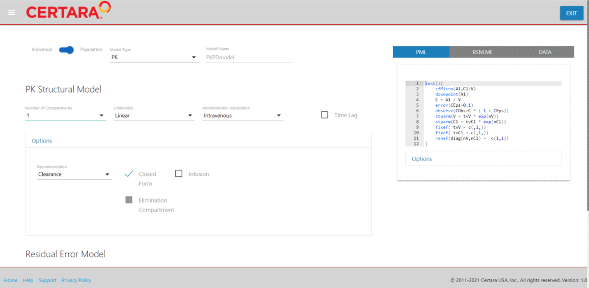
resultsUI(model = baseModel)The series of screenshots below demonstrate how users can preview model diagnostic plots and tables using the tree selection in the Shiny GUI.
Build covariate model
After fitting our baseModel and generating various model
diagnostic plots, let’s begin to introduce covariates.
We will first copy our baseModel using the
copyModel() function, making sure to use the
acceptAllEffects = TRUE argument to accept parameter
estimates from our baseFitJob model execution.
Copying the model not only allows us to accept parameter estimates
across different model runs, but also ensures model output files will be
in separate directories using the modelName argument.
covariateModel <-
  copyModel(baseModel, acceptAllEffects = TRUE,
            modelName = "TwCpt_IVBolus_SelectedCovariateModel_FOCE_ELS")
Next, we’ll add the continuous covariate BodyWeight to
our model and set the covariate effect on structural parameters
V and Cl.
covariateModel <-
  covariateModel %>%
  addCovariate(covariate = "BodyWeight",
               effect = c("V", "Cl"),
               center = "Median")
print(covariateModel)
#>
#>  Model Overview
#>  -------------------------------------------
#> Model Name        :  TwCpt_IVBolus_SelectedCovariateModel_FOCE_ELS
#> Working Directory :  /TestEnvironment/
#> Is population     :  TRUE
#> Model Type        :  PK
#>
#>  PK
#>  -------------------------------------------
#> Parameterization  :  Clearance
#> Absorption        :  Intravenous
#> Num Compartments  :  2
#> Dose Tlag?        :  FALSE
#> Elimination Comp ?:  FALSE
#> Infusion Allowed ?:  FALSE
#> Sequential        :  FALSE
#> Freeze PK         :  FALSE
#>
#>  PML
#>  -------------------------------------------
#> test(){
#>     cfMicro(A1,Cl/V, Cl2/V, Cl2/V2)
#>     dosepoint(A1)
#>     C = A1 / V
#>     error(CEps=0.161251376509829)
#>     observe(CObs=C * ( 1 + CEps))
#>     stparm(V = tvV * ((BodyWeight/median(BodyWeight))^dVdBodyWeight)   * exp(nV))
#>     stparm(Cl = tvCl * ((BodyWeight/median(BodyWeight))^dCldBodyWeight)   * exp(nCl))
#>     stparm(V2 = tvV2)
#>     stparm(Cl2 = tvCl2 * exp(nCl2))
#>     fcovariate(BodyWeight)
#>     fixef( tvV = c(,15.3977961716836,))
#>     fixef( tvCl = c(,6.61266919198735,))
#>     fixef( tvV2 = c(,41.2018786759217,))
#>     fixef( tvCl2 = c(,14.0301337530406,))
#>     fixef( dVdBodyWeight(enable=c(0)) = c(,0,))
#>     fixef( dCldBodyWeight(enable=c(1)) = c(,0,))
#>     ranef(diag(nV,nCl,nCl2) = c(0.069404827604399,0.182196897237991,0.0427782148473702))
#>
#> }
#>
#>  Structural Parameters
#>  -------------------------------------------
#>  V Cl V2 Cl2
#>  -------------------------------------------
#> Observations:
#> Observation Name :  CObs
#> Effect Name      :  C
#> Epsilon Name     :  CEps
#> Epsilon Type     :  Multiplicative
#> Epsilon frozen   :  FALSE
#> is BQL           :  FALSE
#>  -------------------------------------------
#>  Column Mappings
#>  -------------------------------------------
#> Model Variable Name : Data Column name
#> id                  : Subject
#> time                : Act_Time
#> A1                  : Amount
#> BodyWeight          : BodyWeight
#> CObs                : Conc
Note: For continuous covariates, you can center the covariate
value using the center argument in the
addCovariate() function. Options are “Mean”, “Median”,
“Value”, or “None”. By default, center = "None". Depending
on the style argument supplied to the
structuralParameter(), the covariate effect will take a
different functional form. Type
?Certara.RsNLME::structuralParameter and
?Certara.RsNLME::addCovariate for more details.
Investigate covariates inflation
We can investigate the inflation of covariates on different structural parameters using ‘shotgunSearch’ function. It will fit all possible covariates combinations available for the current model. There are 4 scenarios overall (4 combinations of Covariate - Structural parameter relations).
shotgunResults <- shotgunSearch(covariateModel)
print(shotgunResults)
#>                              Scenario RetCode    LogLik     -2LL      AIC
#> 1                            cshot000       1 -632.7954 1265.591 1281.591
#> 2               cshot001 V-BodyWeight       1 -624.4957 1248.991 1266.991
#> 3              cshot002 Cl-BodyWeight       1 -617.2704 1234.541 1252.541
#> 4 cshot003 V-BodyWeight Cl-BodyWeight       1 -608.6464 1217.293 1237.293
#>        BIC nParm nObs nSub EpsShrinkage Condition
#> 1 1303.339     8  112   16      0.17365   4.84292
#> 2 1291.458     9  112   16      0.14411   9.62860
#> 3 1277.007     9  112   16      0.16187   8.17619
#> 4 1264.478    10  112   16      0.13193  19.88073
The minimal -2LL value observed for combination with both relationships (V-BodyWeight and Cl-BodyWeight) included. Note that for ‘shotgunSearch()’, as well as for other job-parallelized functions like ‘bootstrap()’, ‘stepwiseSearch()’, ‘sortfit()’ the default host (hostPlatform argument) is multicore with 4 cores:
MulticoreLocalHost <- hostParams(
  installationDirectory = Sys.getenv("INSTALLDIR"),
  parallelMethod = "multicore",
  hostName = "multicore4",
  numCores = 4
)
That approach (by job parallelization) is effective way to speed up the computation of these runs. Multiple jobs are started at once. In doing so, the user delegates to the system a job distribution process across all available cores, just providing the number of jobs/processes not to be exceeded with current run (numCores argument). It is not recommended to specify the number in ‘numCores’ exceeding the number of cores of CPU(s) available.
Fit covariate model
covariateFitJob <- fitmodel(covariateModel)
print(covariateFitJob$Overall)
#>    Scenario RetCode    LogLik     -2LL      AIC      BIC nParm  nObs  nSub
#>      <char>   <int>     <num>    <num>    <num>    <num> <int> <int> <int>
#> 1: WorkFlow       1 -608.6464 1217.293 1237.293 1264.478    10   112    16
#>    EpsShrinkage Condition
#>           <num>     <num>
#> 1:      0.13193  19.88073
Generate covariate model diagnostics
Just like we did for our baseModel, we’ll use the
Certara.Xpose.NLME package to import results of
fitmodel() into an xpose_data object and use
functions from the Certara.Xpose.NLME package to generate
our covariate model diagnostic plots.
library(Certara.Xpose.NLME)
library(xpose)

covariateModel_xpdb <-
  xposeNlmeModel(covariateModel,covariateFitJob)
Create model diagnostic plots for our
covariateModel.
CWRES vs BodyWeight
covariateModel_xpdb %>%
  res_vs_cov(
    type = "ps",
    res = "CWRES",
    covariate = "BodyWeight",
    caption = "/TwCpt_IVBolus_SelectedCovariateModel_FOCE_ELS"
  )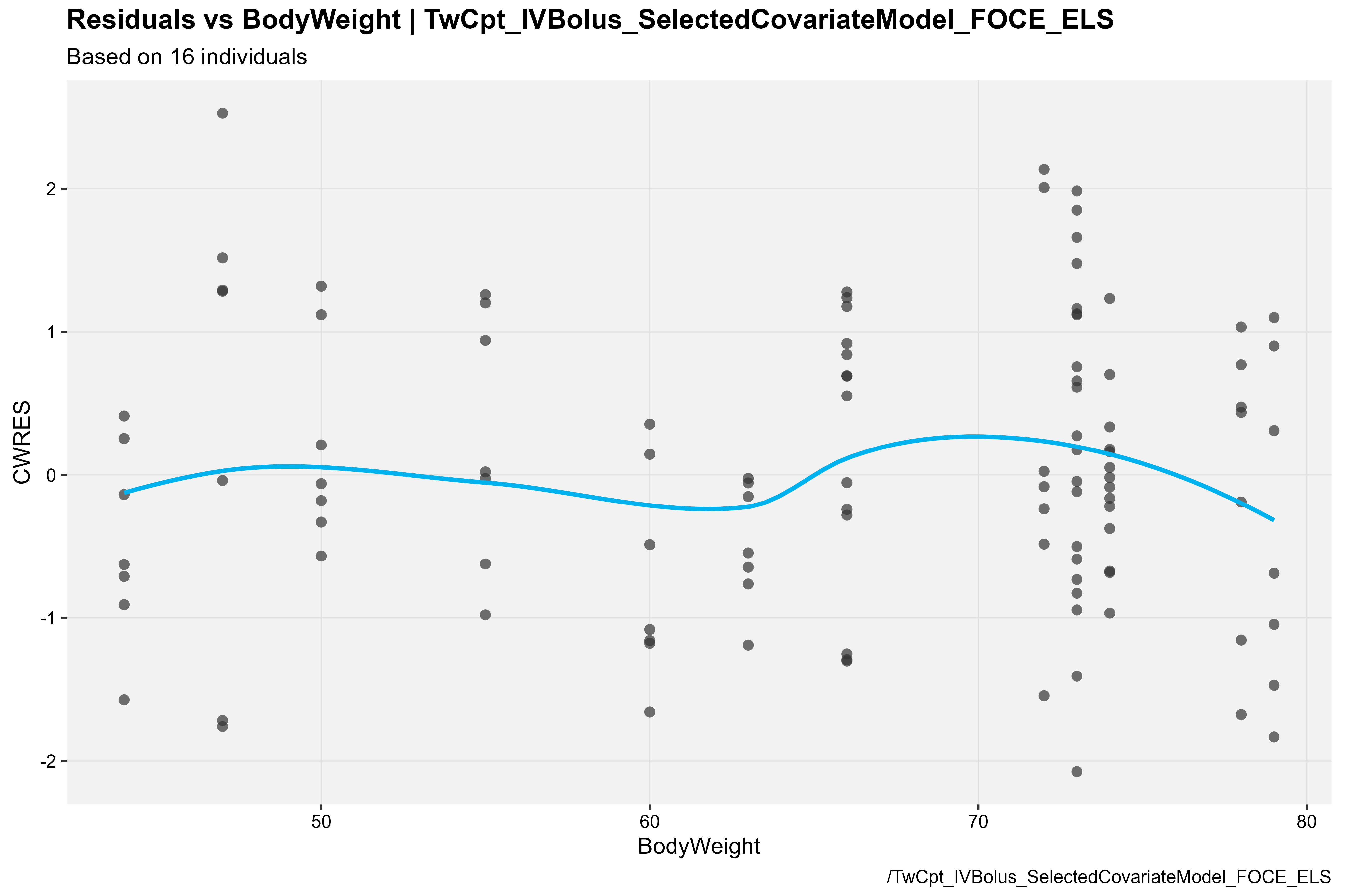
Note: The above covariate plot is available in the
Certara.Xpose.NLME package v1.1.0. If using
v1.0.0, please type
?Certara.Xpose.NLME::nlme.var.vs.cov for CWRES vs covariate
usage details.
ETA vs BodyWeight
covariateModel_xpdb %>%
  eta_vs_cov(type = "ps", covariate = "BodyWeight",
caption = "/TwCpt_IVBolus_SelectedCovariateModel_FOCE_ELS") 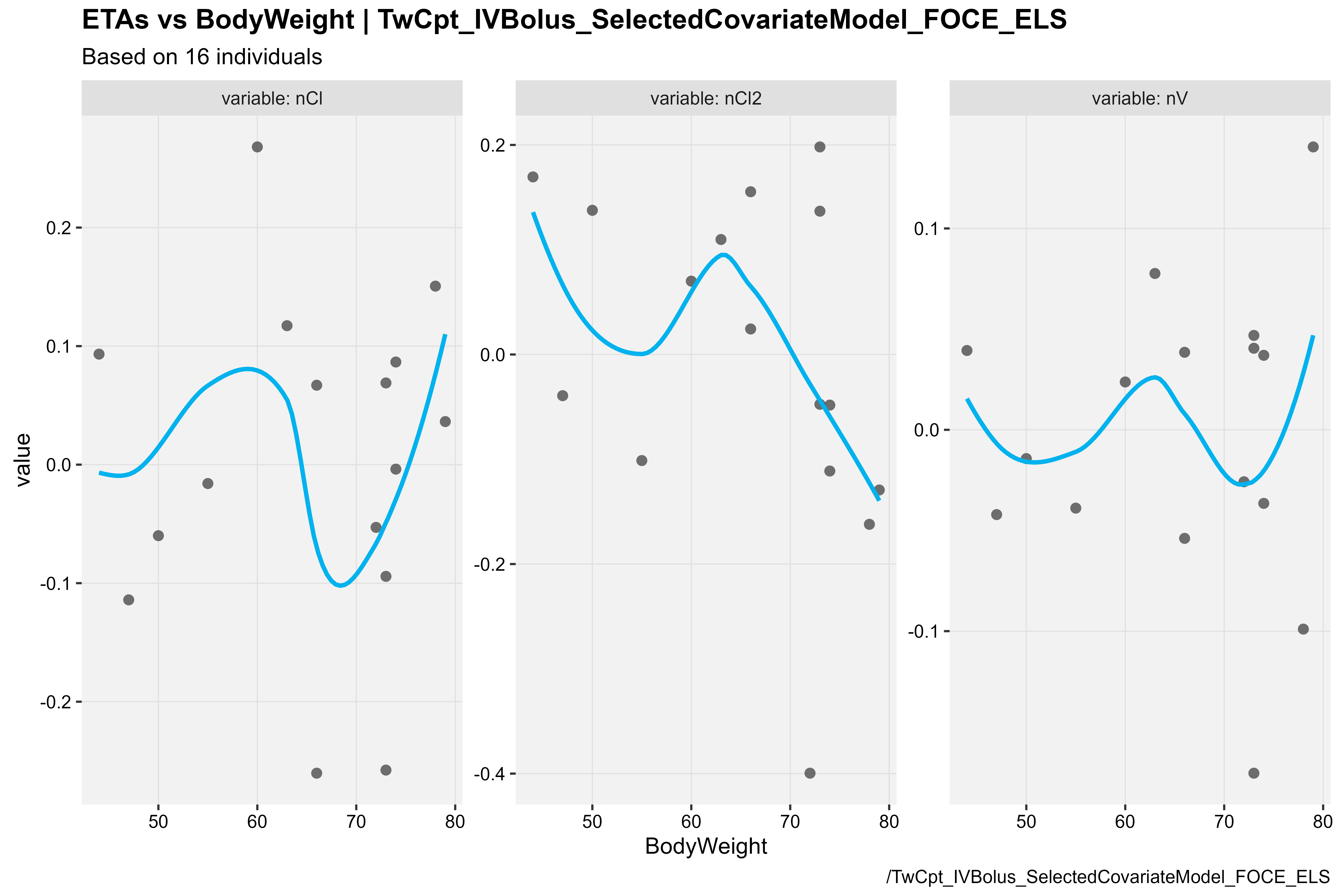
Launch resultsUI() with base and covariate models
Finally, we can pass a vector of our model objects to the
model argument in resultsUI() and initiate the
Shiny GUI with both of our models. This will allow us to easily compare
the same model diagnostics plots and tables across models and generate R
code for any model diagnostics we may want to reproduce at a later
time.
For more details, see Certara.ModelResults website.
library(Certara.ModelResults)

resultsUI(model = c(baseModel, covariateModel))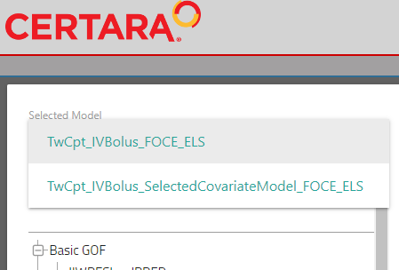
Perform VPC analysis for covariate model
After generating various model diagnostic plots and tables, we may want to generate a Visual Predictive Check (VPC) next.
Repeating what we did when we copied our covariateModel
from our baseModel, we will use the
copymodel() function to create a new model object with a
new run directory, then execute our new model using the
vpcmodel() function.
covariateModelVPC <-
  copyModel(covariateModel,
            acceptAllEffects = TRUE,
            modelName = "VPC_TwCpt_IVBolus_SelectedCovariateModel")
Execute vpcmodel() function.
covariateVPCJob <- vpcmodel(covariateModelVPC)Generate VPC diagnostics
To generate our VPC using the tidyvpc package, we can
extract the observed and simulated data from the return value of the
vpcmodel() function. Additionally, the observed data file
for continuous observed variables is saved as
predcheck0.csv and the simulated data file as
predout.csv in the model output directory (e.g.,
covariateModel@modelInfo@workingDir).
For more details on syntax, see the tidyvpc website.
obs <- covariateVPCJob$predcheck0

sim <- covariateVPCJob$predout
Next, we’ll generate both a binned and binless VPC using the
tidyvpc package.
For our binned VPC, we’ll specify the pam binning method
with 8 bins.
library(tidyvpc)

binned_VPC <- observed(obs, x = IVAR, yobs = DV) %>%
  simulated(sim, ysim = DV) %>%
  binning(bin = "pam", nbins = 8) %>%
  vpcstats()


plot(binned_VPC)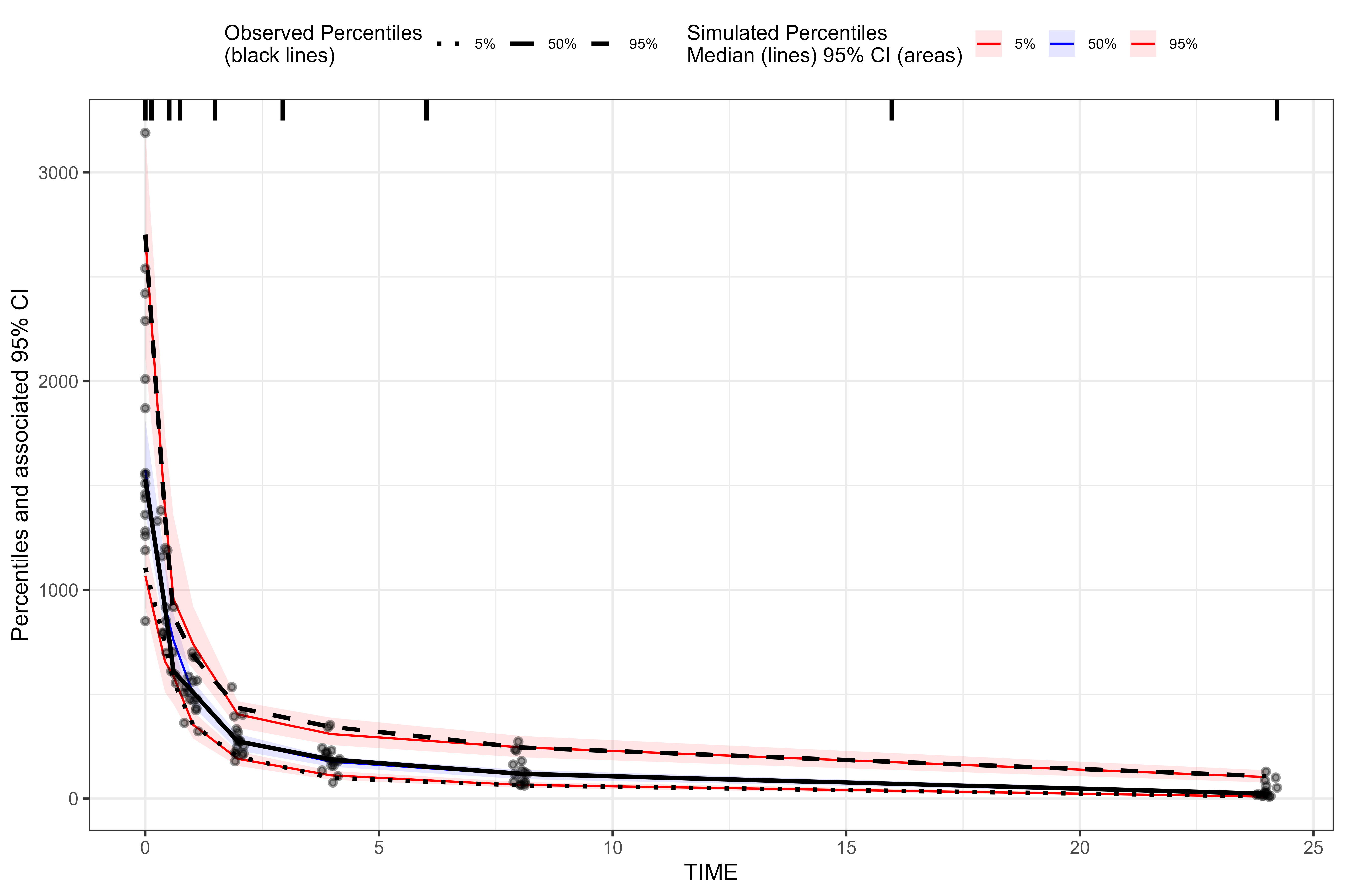
For our binless VPC, we’ll automatically optimize the lambda
smoothing parameters (in the additive quantile regression based on AIC)
by setting optimize = TRUE in the binless()
function.
binless_VPC <-
  observed(obs, x = IVAR, yobs = DV) %>%
  simulated(sim, ysim = DV) %>%
  binless(optimize = TRUE) %>%
  vpcstats()

plot(binless_VPC)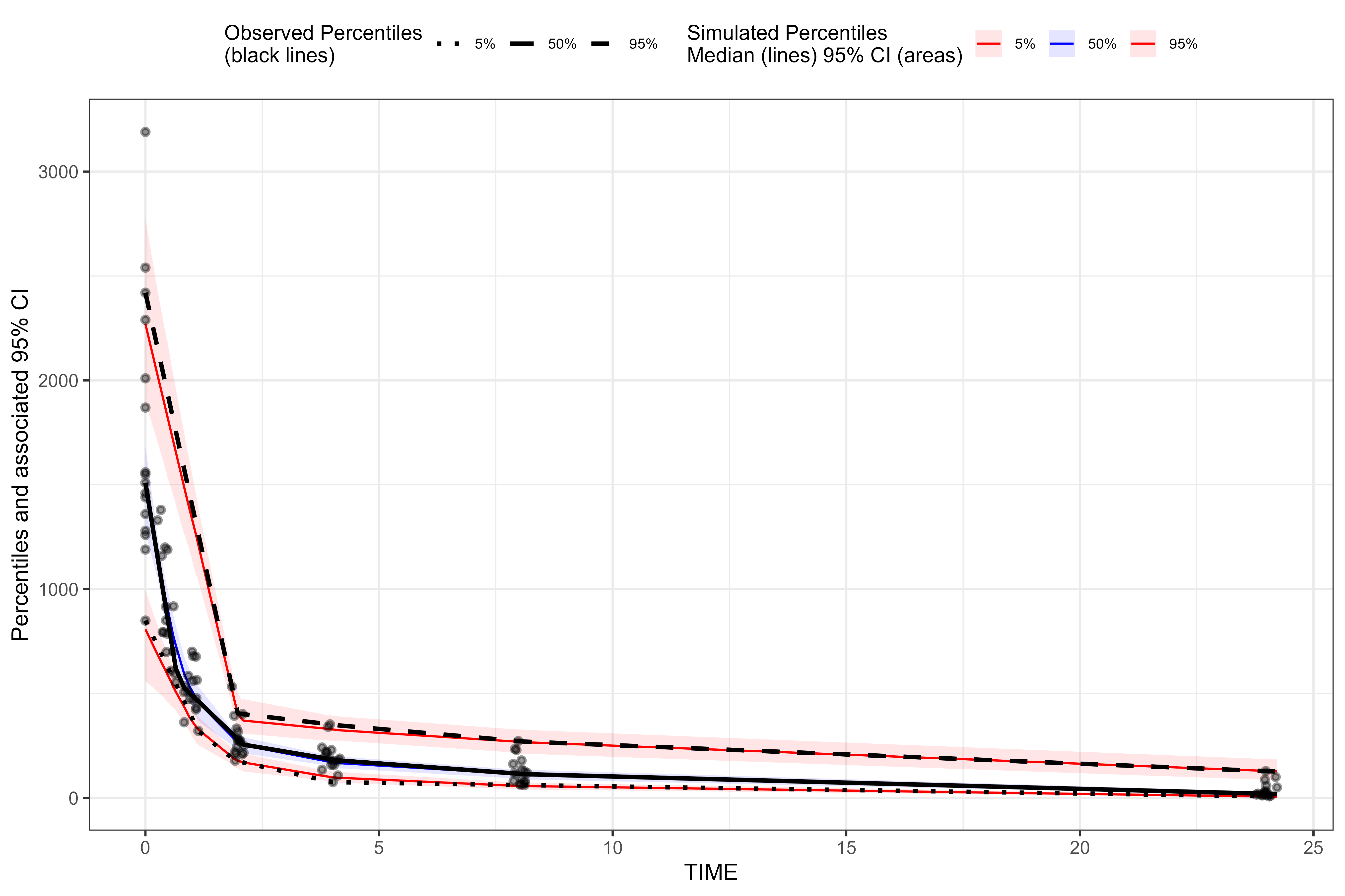
We can see that the results of the traditional binned VPC resemble the results of the binless VPC. For more details about the binless methodology, see A Regression Approach to Visual Predictive Checks for Population Pharmacometric Models.
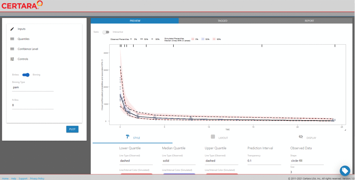
Launch vpcResultsUI()
The Certara.VPCResults package provides a Shiny
interface to parameterize Visual Predictive Checks (VPC) and generate
corresponding tidyvpc and ggplot2 code to
reproduce the VPC from R. Users can tag multiple VPC plots of
interest in the Shiny session, and render plots into a report, or
generate the raw .R or .Rmd files to reproduce
VPCs and ggplot2 output from R.
library(Certara.VPCResults)

vpcResultsUI(obs, sim)