Overview
R Speaks Non Linear Mixed Effects Modeling, RsNLME, is a suite of R packages and supplementary Shiny apps developed by Certara that supports pharmacometric modeling inside R.
When used together, these packages can add a level of speed and flexibility to your pharmacometrics workflow that cannot be achieved with point-and-click type tools.
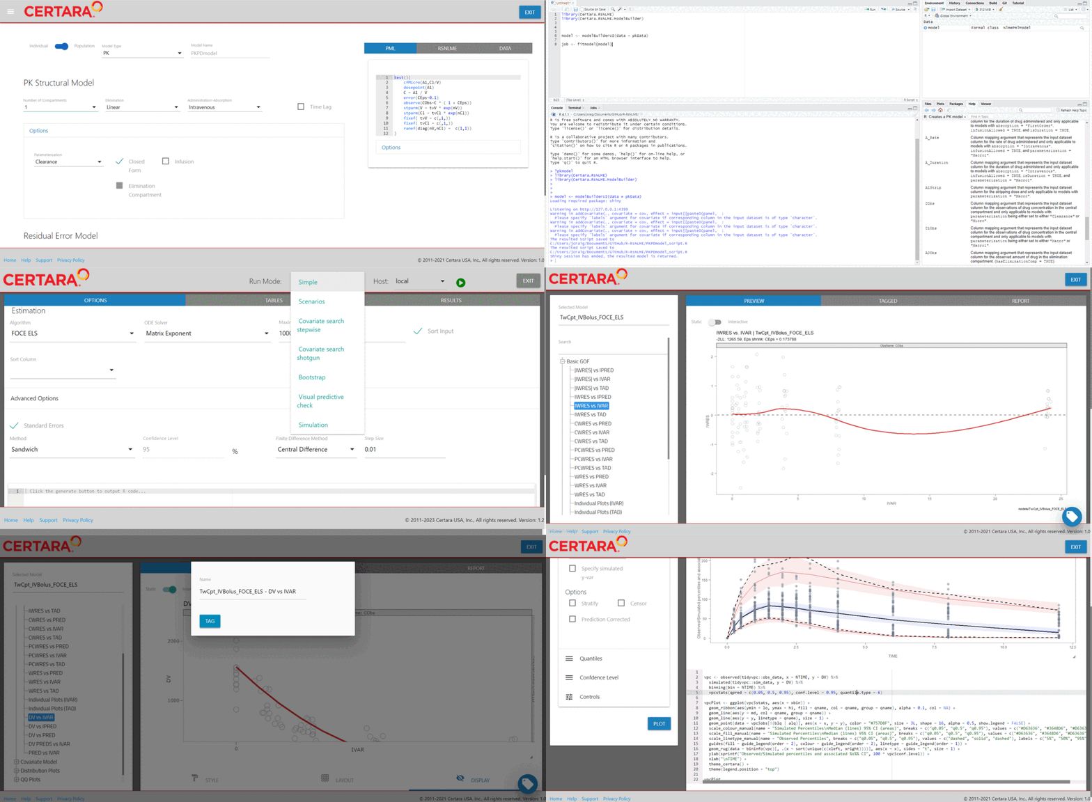
Whether you’re still learning R or a seasoned expert, efficiently build, execute, and analyze your models from the Shiny GUI, then generate the corresponding R code to reproduce and expand your workflow from the R command line.

Usage
Certara.RsNLME uses tidyverse syntax to generate and update pharmacometric models in R. All functions can easily be chained together using the %>% operator from magrittr. See RsNLME Examples.
library(Certara.RsNLME)
library(magrittr)


# Create two-compartment pharmacokinetic model
model <- pkmodel(numCompartments = 2, data = pkData,
                ID = "Subject", Time = "Act_Time", A1 = "Amount", CObs = "Conc",
                modelName = "TwCpt_IVBolus_FOCE_ELS")


# Update initial estimates
model <- model %>%
          fixedEffect(effect = c("tvV", "tvCl", "tvV2", "tvCl2"), value = c(15, 5, 40, 15))
Model Builder
If you are still learning the command line syntax, use the Certara.RsNLME.ModelBuilder Shiny application from either RStudio or Pirana to build your NLME model from the GUI and generate the corresponding R and PML code to reproduce your model across multiple environments.
library(Certara.RsNLME)
library(Certara.RsNLME.ModelBuilder)

model <- modelBuilderUI(data = pkData)
Learn more about Certara.RsNLME.ModelBuilder here
Fit model
Next, we can execute the above model we created from the Shiny GUI inside R using the command fitmodel():
Model Executor
Or alternatively, use the Certara.RsNLME.ModelExecutor Shiny application to specify additional engine arguments, change the estimation algorithm, add output tables, and more - all from the Shiny GUI!
Learn more about Certara.RsNLME.ModelExecutor here
Xpose NLME
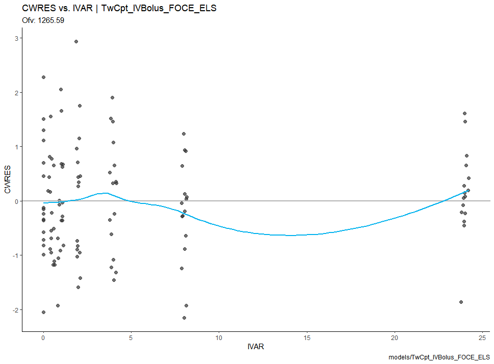
After executing the model, we use the Certara.Xpose.NLME, xpose, ggplot2, and flextable packages to generate our model diagnostic plots.
library(Certara.Xpose.NLME)
library(xpose)
library(ggplot2)

xpdb <- xposeNlmeModel(model, job)

res_vs_idv(xpdb) +
   theme_classic()
Learn more about Certara.Xpose.NLME here
Model Results
Or alternatively, use the Certara.ModelResults Shiny application to easily preview, customize, and report model diagnostics plots and tables from the Shiny GUI. Furthermore, the application will generate the corresponding .R and .Rmd code to reproduce your model diagnostics.
library(Certara.ModelResults)

resultsUI(model)
Learn more about Certara.ModelResults here
Fit VPC model
Lastly, users can execute a vpcmodel() to generate a Visual Predictive Check (VPC) plot and assess model fit.
Using the Certara.RsNLME package, we will execute the function vpcmodel() to return our observed and simulated data used to generate our VPC.
library(Certara.RsNLME)

vpcJob <- vpcmodel(model)
Next we’ll extract our observed and simulated data from the return value of vpcmodel().
obs_data <- vpcJob$predcheck0

sim_data <- vpcJob$predout
tidyvpc
Then we can use the tidyvpc package to parameterize our VPC.
library(tidyvpc)

 vpc <- observed(obs_data, y = DV, x = IVAR) %>%
      simulated(sim_data, y = DV) %>%
      binless() %>%
      vpcstats()
Learn more about tidyvpc here
VPC Results
Or alternatively, use the Certara.VPCResults Shiny application to easily parameterize, customize, and report VPC plots from the Shiny GUI. Furthermore, the application will generate the corresponding .R and .Rmd code to reproduce your VPC’s in R.
vpcResultsUI(obs_data, sim_data)Learn more about Certara.VPCResults here
