Absorption Delay Models in RsNLME • Certara.RsNLME

RsNLME package logo

Overview

The purpose of this vignette is to demonstrate how to create an absorption delay model through built-in model library, fit the model, create commonly used diagnostic plots through both command-line and mode results shiny app (from Certara.ModelResults package), perform VPC and create VPC plots through tidyvpc package (command-line) or VPC results shiny app from Certara.VPCResults package.

The model demonstrated is a one-compartment model with 1st-order clearance and the delay time between the administration time of the drug and the time when the drug molecules reach the central compartment is assumed to be gamma distributed. In other words, the model is described as follows: $\frac{dA1(t)}{dt} = \sum_{i=1}^{m}D_{i} gammaPDF(t - t_{Di}; rateParameter, shapeParameter) - Cl/V * A1(t)$

where

$A1$ denotes the drug amount at central compartment with $V$ and $Cl$ respectively being the central volume distribution and central clearance rate
$m$ denotes the number of bolus dosing events
$D_{i}$ is the amount of dose administered at time $t_{Di}$ for the ith dosing events
gammaPDF denotes the probability density function of a gamma distribution with with $mean = MeanDelayTime$ and shape parameter being $(ShapeParamMinusOne + 1)$

(For more information on distribute delays, please visit here).

For the rest of this document, we assume that all the necessary packages are loaded and the directory with NLME Engine is given as an environment variable (INSTALLDIR). They can be loaded and checked with the following commands:

# loading the package
library(Certara.RsNLME)
library(data.table)
library(dplyr)
library(xpose)
library(Certara.Xpose.NLME)
library(ggplot2)
library(Certara.ModelResults)
library(Certara.VPCResults)
library(tidyvpc)

# Check the environment variable
Sys.getenv("INSTALLDIR")

Create the model

We will use the input dataset OneCpt_GammaDistributedAbsorptionDelay.csv included with the Certara.RsNLME package.

filename <- system.file("vignettesdata/OneCpt_GammaDistributedAbsorptionDelay.csv",
                        package = "Certara.RsNLME",
                        mustWork = TRUE)
dt_InputDataSet <- fread(filename)

Next, we will define a one-compartment model with gamma absorption delay and 1st-order clearance and make the following modifications to it:

Set $V = e^{tvlogV + nlogV}$
Set $Cl = e^{tvlogCl + nlogCl}$
Set $MeanDelayTime = e^{tvlogMeanDelayTime + nlogMeanDelayTime}$
Set $ShapeParamMinusOne = e^{tvlogShapeParamMinusOne}$
Change initial values for fixed effects $tvlogV$ and $tvlogShapeParamMinusOne$ to be 5 and 2, respectively (the default value is 1)
Add secondary parameter $tvV$ , which is set to $tvV = e^{tvlogV}$
Add secondary parameter $tvCl$ , which is set to $tvCl = e^{tvlogCl}$
Add secondary parameter $tvMeanDelayTime$ , which is set to $tvMeanDelayTime = e^{tvlogMeanDelayTime}$
Add secondary parameter $tvShapeParam$ , which is set to $tvShapeParam = e^{tvlogShapeParamMinusOne} + 1$

model <- pkmodel(absorption = "Gamma"
                 , data = dt_InputDataSet
                 , columnMap = FALSE
                 , modelName = "OneCpt_GammaDistributedAbsorptionDelay"
                 ) %>%
structuralParameter(paramName = "V", 
                    style = "LogNormal2", 
                    fixedEffName = "tvlogV", 
                    randomEffName = "nlogV") %>%
structuralParameter(paramName = "Cl", 
                    style = "LogNormal2", 
                    fixedEffName = "tvlogCl", 
                    randomEffName = "nlogCl") %>%
structuralParameter(paramName = "MeanDelayTime", 
                    style = "LogNormal2", 
                    fixedEffName = "tvlogMeanDelayTime", 
                    randomEffName = "nlogMeanDelayTime") %>%
structuralParameter(paramName = "ShapeParamMinusOne", 
                    style = "LogNormal2", 
                    fixedEffName = "tvlogShapeParamMinusOne", 
                    hasRandomEffect = FALSE) %>%
fixedEffect(effect = c("tvlogV", "tvlogShapeParamMinusOne"), value = c(5, 2)) %>%
addSecondary(name = "tvV", definition = "exp(tvlogV)") %>%
addSecondary(name = "tvCl", definition = "exp(tvlogCl)") %>%
addSecondary(name = "tvMeanDelayTime", definition = "exp(tvlogMeanDelayTime)") %>%
addSecondary(name = "tvShapeParam", definition = "exp(tvlogShapeParamMinusOne) + 1")

Let’s view the model and its associated column mappings, and then map those un-mapped model variables to their corresponding input data columns:

print(model)

 Model Overview 
 ------------------------------------------- 
Model Name        :  OneCpt_GammaDistributedAbsorptionDelay
Working Directory :  /TestEnvironment/
Is population     :  TRUE
Model Type        :  PK

 PK 
 ------------------------------------------- 
Parameterization  :  Clearance
Absorption        :  Gamma
Num Compartments  :  1
Dose Tlag?        :  FALSE
Elimination Comp ?:  FALSE
Infusion Allowed ?:  FALSE
Sequential        :  FALSE
Freeze PK         :  FALSE

 PML 
 ------------------------------------------- 
test(){
    dosepoint(A1)
    C = A1 / V
    delayInfCpt(A1, MeanDelayTime, ShapeParamMinusOne, out =  -  Cl * C, dist = Gamma)
    error(CEps=0.1)
    observe(CObs=C * ( 1 + CEps))
    stparm(MeanDelayTime = exp(tvlogMeanDelayTime + nlogMeanDelayTime))
    stparm(ShapeParamMinusOne = exp(tvlogShapeParamMinusOne ))
    stparm(V = exp(tvlogV + nlogV))
    stparm(Cl = exp(tvlogCl + nlogCl))
    fixef( tvlogMeanDelayTime = c(,1,))
    fixef( tvlogShapeParamMinusOne = c(,2,))
    fixef( tvlogV = c(,5,))
    fixef( tvlogCl = c(,1,))
    ranef(diag(nlogMeanDelayTime,nlogV,nlogCl) = c(1,1,1))
    secondary(tvV=exp(tvlogV))
    secondary(tvCl=exp(tvlogCl))
    secondary(tvMeanDelayTime=exp(tvlogMeanDelayTime))
    secondary(tvShapeParam=exp(tvlogShapeParamMinusOne) + 1)
}

 Structural Parameters 
 ------------------------------------------- 
 MeanDelayTime ShapeParamMinusOne V Cl
 ------------------------------------------- 
Observations:
Observation Name :  CObs
Effect Name      :  C
Epsilon Name     :  CEps
Epsilon Type     :  Multiplicative
Epsilon frozen   :  FALSE
is BQL           :  FALSE
 ------------------------------------------- 
 Column Mappings 
 ------------------------------------------- 
Model Variable Name : Data Column name
id                  : ID
time                : Time
A1                  : ?
CObs                : CObs

## Manually map those un-mapped model variables 
## to their corresponding input data columns
model <- model %>% colMapping(c(A1 = "Dose"))

Model Fitting

Let’s run the model using the fitmodel function with default host and engine method set to be QRPEM.

job <- fitmodel(model, method = "QRPEM")

print(job$Overall)
   Scenario RetCode   LogLik      -2LL       AIC       BIC nParm nObs nSub
1: WorkFlow       1 685.0575 -1370.115 -1354.115 -1317.481     8  720   80
   EpsShrinkage Condition
1:      0.14701   2.50109

Diagnostic Plots

We will use the xposeNlme function from the Certara.Xpose.NLME package to import estimation results to xpose database to create some commonly used diagnostic plots. Majority of the plotting functions provided in the xpose package can be used. Here we only demonstrate several of these functions.

## Imports results of an NLME run into xpose database to create
## commonly used diagnostic plots
xp <-
  xposeNlme(dir = model@modelInfo@workingDir, 
            modelName = "OneCpt_GammaDistributedAbsorptionDelay")

## observations against population predictions
dv_vs_pred(xp,
           type = "p",
           subtitle = "-2LL: @ofv",
           caption = "dv_vs_pred")


## observations against individual predictions
dv_vs_ipred(xp,
            type = "p",
            subtitle = "-2LL: @ofv, Eps shrinkage: @epsshk",
            caption = "dv_vs_ipred")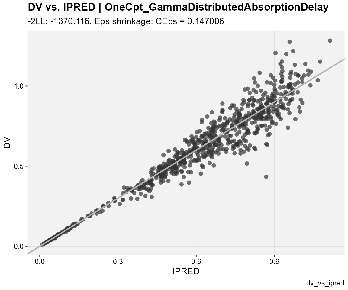


## CWRES against population predictions
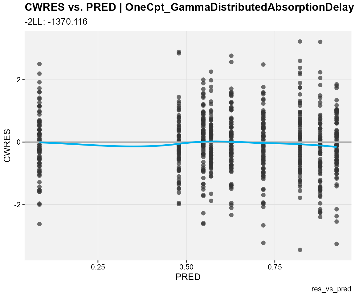
res_vs_pred(
  xp,
  res = "CWRES",
  type = "ps",
  subtitle = "-2LL: @ofv",
  caption = "res_vs_pred"
)


## CWRES against the independent variable
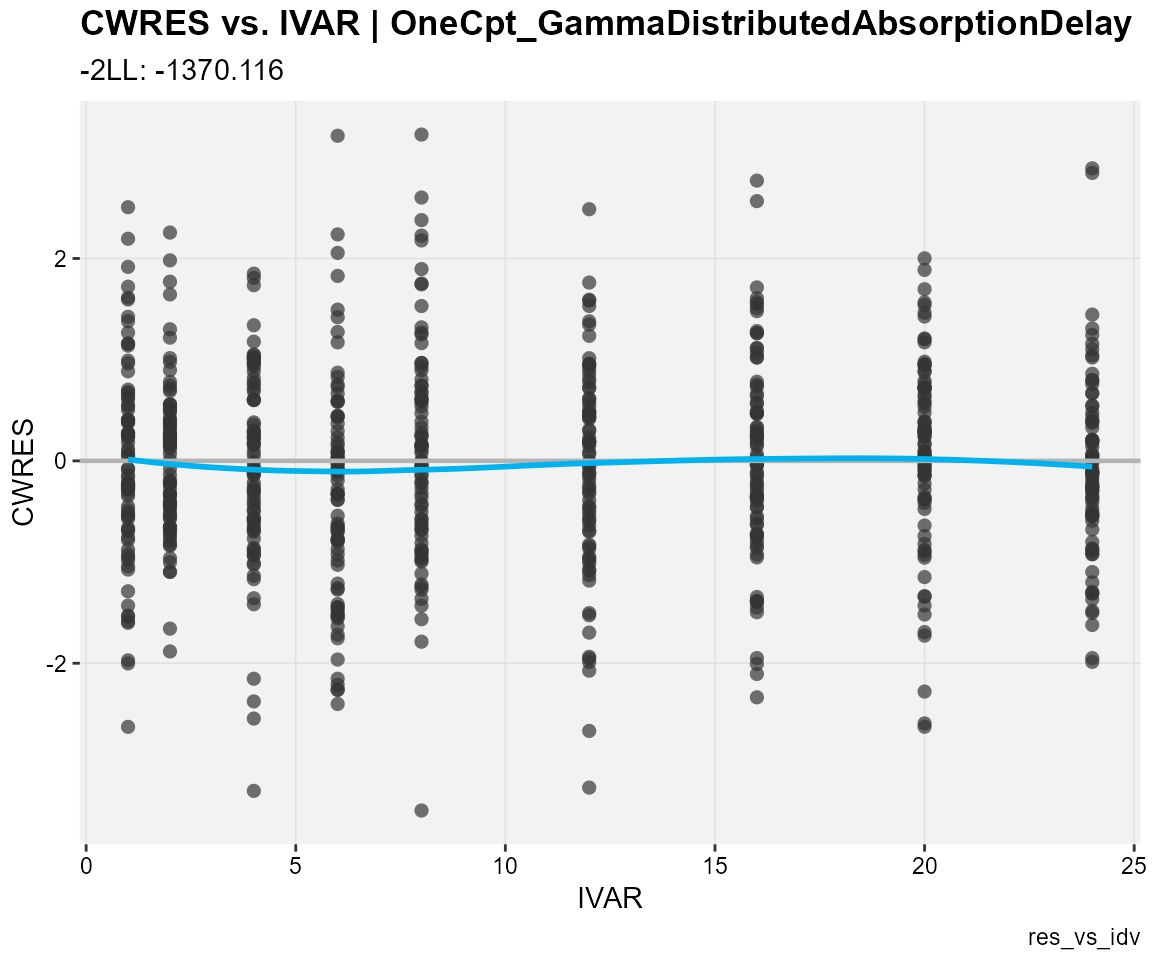
res_vs_idv(
  xp,
  res = "CWRES",
  type = "ps",
  subtitle = "-2LL: @ofv",
  caption = "res_vs_idv"
)


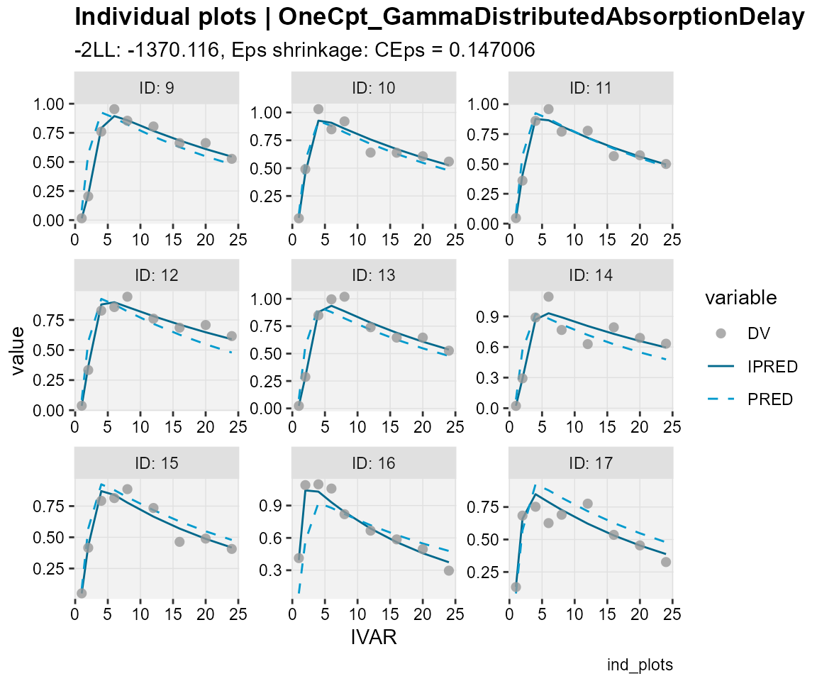
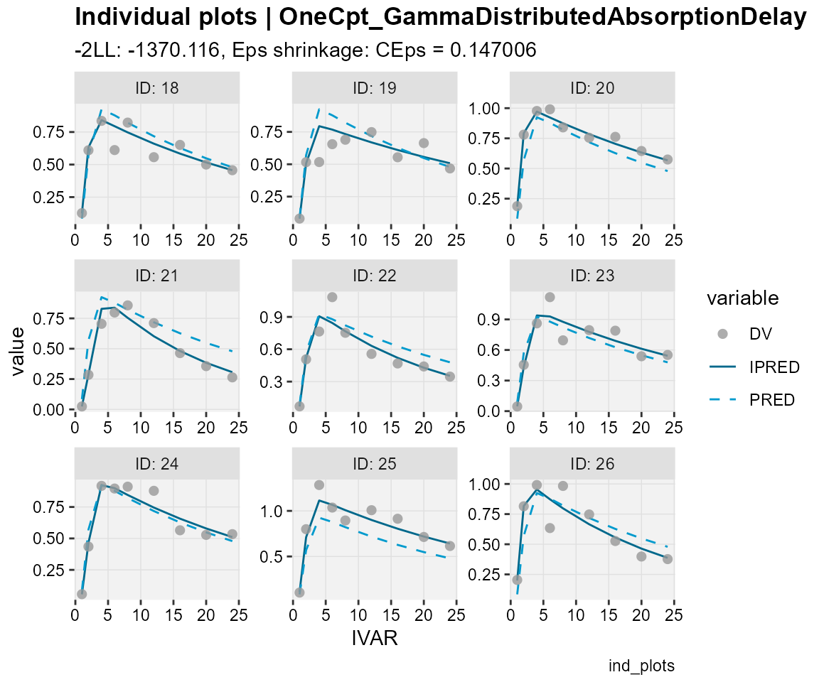
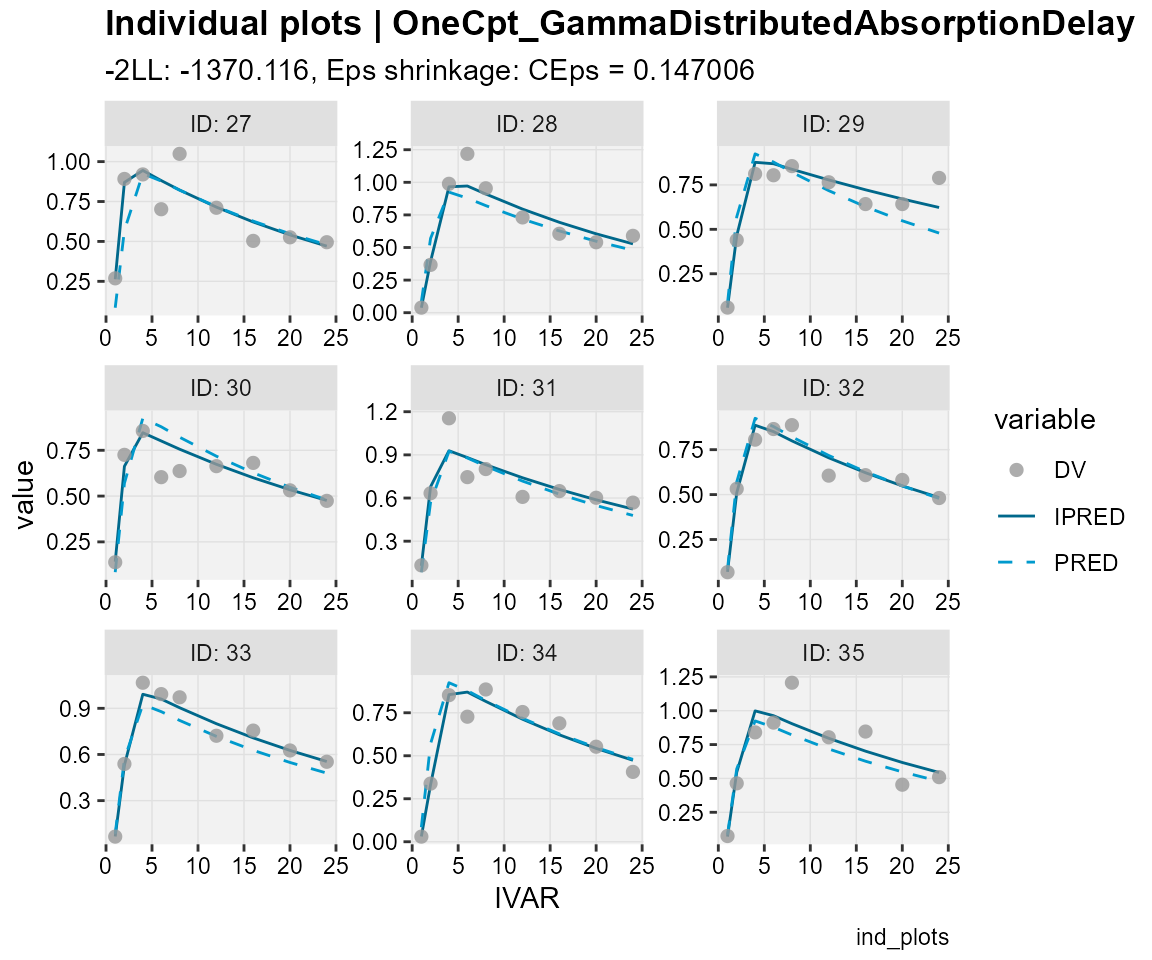
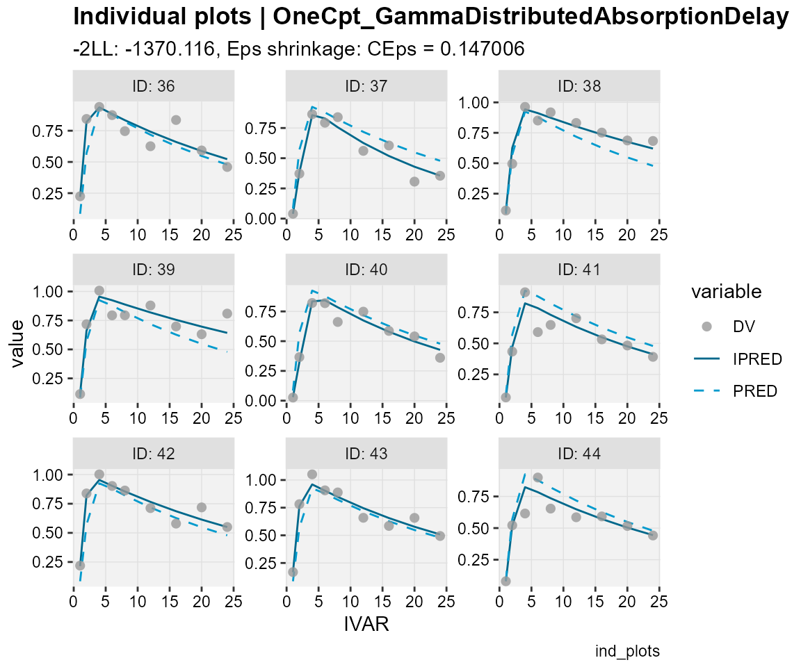
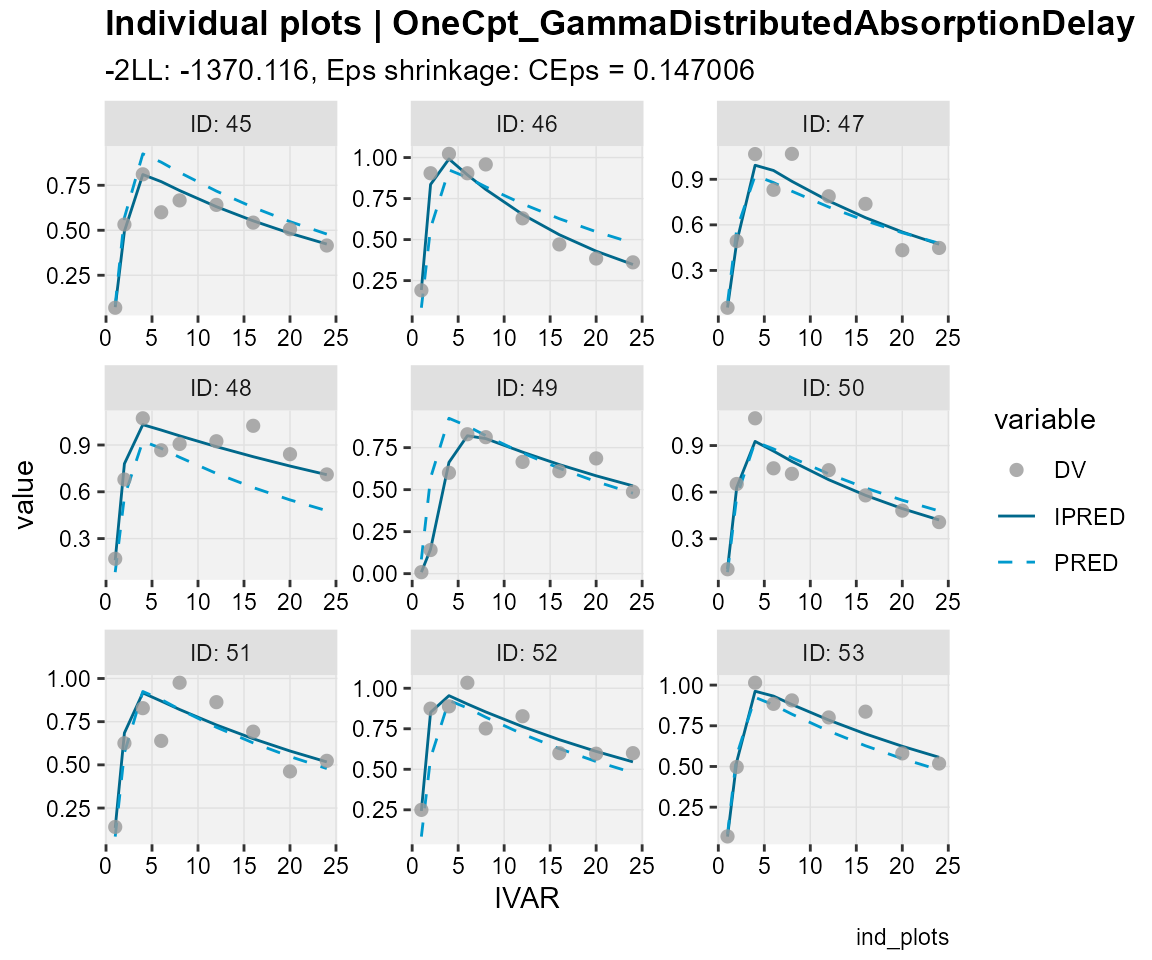
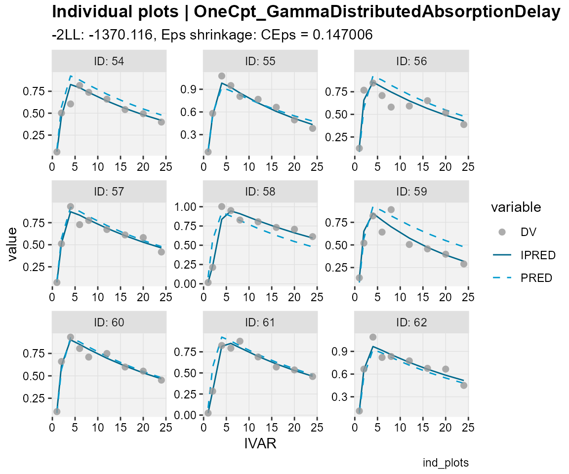
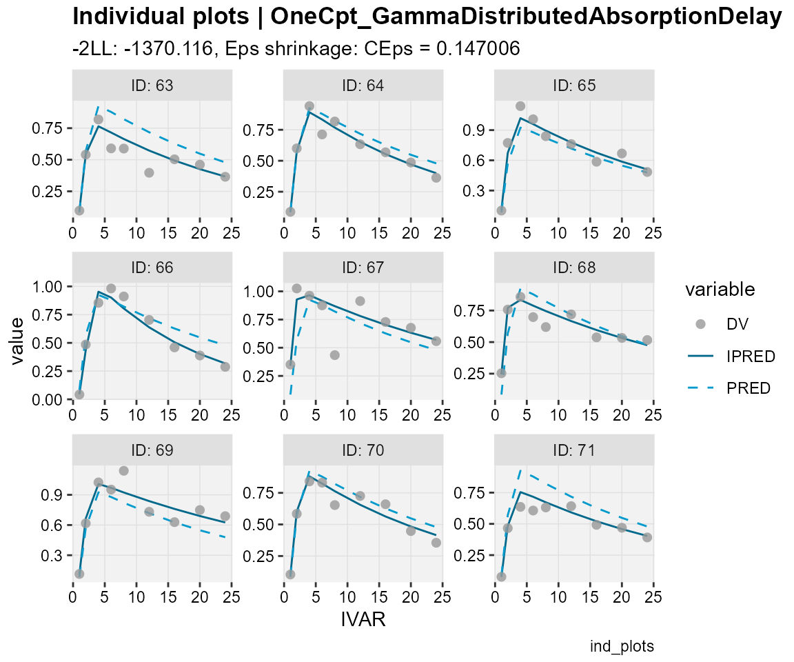
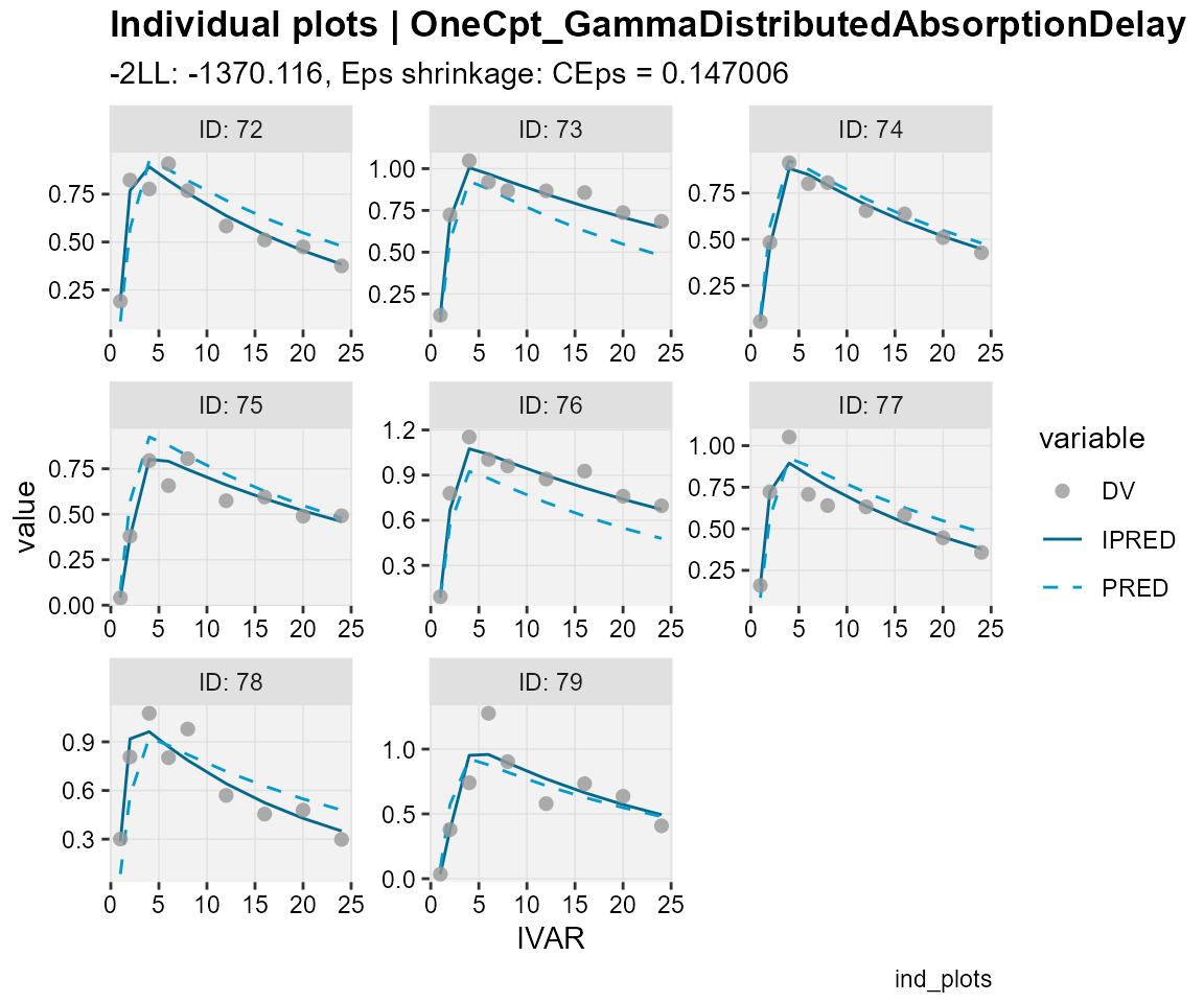
## Observations, individual predictions and population predictions
## plotted against the independent variable for every individual
ind_plots(xp, 
          subtitle = "-2LL: @ofv, Eps shrinkage: @epsshk", 
          caption = "ind_plots")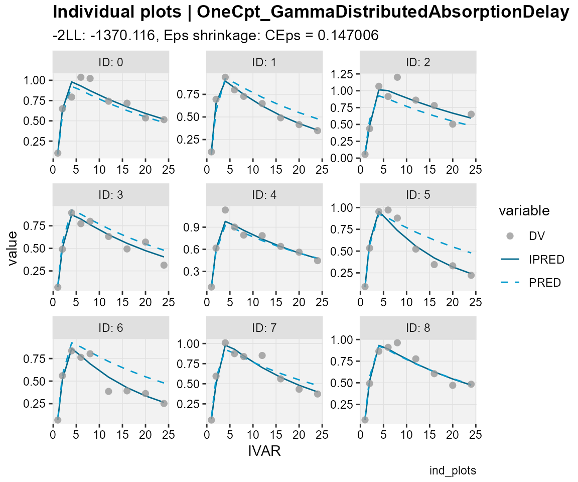


## create diagnostic plots to assess the distribution 
## of individual random effects (ETA values)
eta_distrib(xp, 
            caption = "eta_distrib")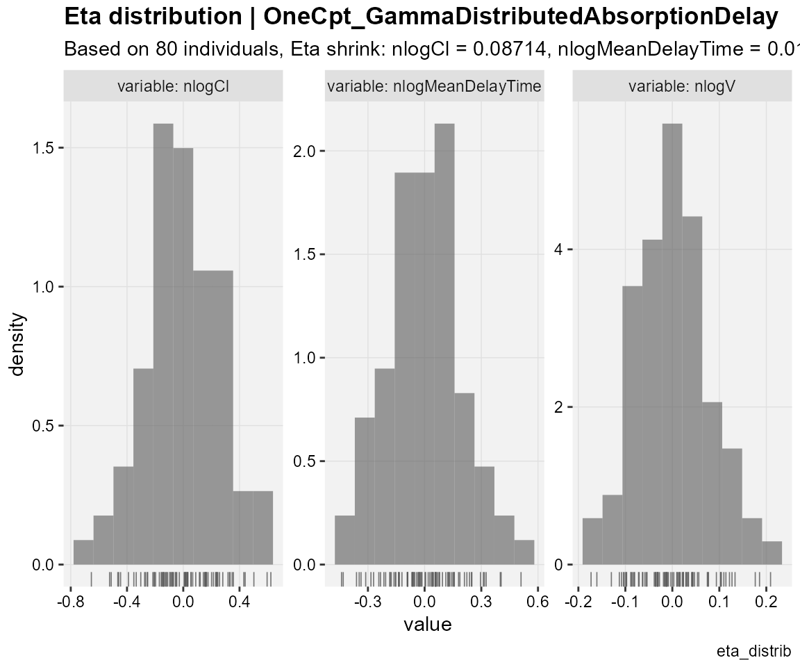

Alternatively, one can view/customize diagnostic plots as well as estimation results through model results shiny app (from the Certara.ModelResults package), which can also be used to generate R script and report as well as the associated R script and report as well as the associated R markdown. For details on this app as well as how to use it, please visit the following link. Here we only demonstrate how to invoke this shiny app through either model object or the xpose data bases created above.


## Invoke model results shiny app through model object defined above 
resultsUI(model)

## Or invoke model results shiny app through xpose database created above 
resultsUI(xpdb = xp)

VPC

We will use the copyModel function to copy model into a new object and accept final parameter estimates from fitting run as initial estimates for VPC simulation:


modelVPC <- 
  copyModel(model, 
            acceptAllEffects = TRUE, 
            modelName = "OneCpt_GammaDistributedAbsorptionDelay_VPC")

Now, let’s run VPC using the vpcmodel function with the default host, default values for the relevant NLME engine arguments, and default values for VPC arguments:

vpcJob <- vpcmodel(modelVPC)

## Observed data
dt_ObsData <- vpcJob$predcheck0

## Simulated data
dt_SimData <- vpcJob$predout

Next, we will create VPC plots through tidyvpc package. The tidyvpc package provides support for both continuous and categorical VPC using both binning and binless methods. For details on this package, please visit the following link. Note that this example only contains one observed variable and both simulated and observed data meet the requirements set by tidyvpc package. Hence, there is no need to do any data preprocessing for this example.

## Create a binless VPC plot 
plot_binless_vpc <- observed(dt_ObsData, x = IVAR, yobs = DV) %>%
  simulated(dt_SimData, ysim = DV) %>%
  binless() %>%
  vpcstats()
plot(plot_binless_vpc)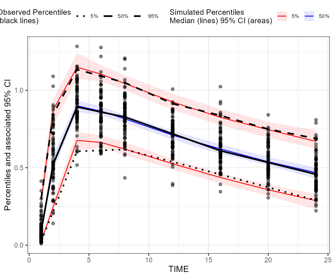


## Create a binning VPC plot: binning on x-variable itself 
plot_binning_vpc <- observed(dt_ObsData, x = IVAR, yobs = DV) %>%
  simulated(dt_SimData, ysim = DV) %>%
  binning(bin = IVAR) %>%
  vpcstats()
plot(plot_binning_vpc)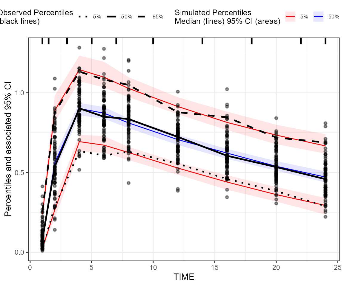

Alternatively, one can create/customize VPC plots through VPC results shiny app (from Certara.VPCResults package), which can also be used to:

generate corresponding tidyvpc code to reproduce the VPC ouput from R command line
generate report as well as the associated R markdown.

Here we only demonstrate how to invoke this shiny app:

  vpcResultsUI(observed = dt_ObsData, simulated = dt_SimData)