Simulation in RsNLME

Overview

The purpose of this vignette is to demonstrate how to edit a build-in model and then simulate it.

The model demonstrated is a two-compartment model with an IV bolus. It involves both plasma and urine compartments with the urine compartment reset to zero right after each observation.

Create the model

It is assumed that directory with NLME Executables is given as an environment variable (INSTALLDIR), which can be checked with the following commands:

  # loading the package
  library(Certara.RsNLME)
  library(data.table)
  library(ggplot2)
  library(dplyr)

 # Check the environment variable
  Sys.getenv("INSTALLDIR")
[1] "C:\\Program Files\\Certara\\NLME_Engine"

First we will create the simulation input dataset

  dt_SimInputData <- data.table(ID = c(1, 2), Time = 0, Dose = c(10, 20))

Next, we will define the model and the associate column mappings:

• Create a basic two-compartment PK model with IV bolus and define the associated column mappings
• Change initial values for fixed effects tvV, tvV2, and tvCl2, to 5, 3, 0.5, respectively
• Change the covariance matrix of random effects to be a diagonal matrix with all the diagonal elements being 0.1
• Change the standard deviation of residual error variable corresponding to observed variable A0Obs to 0.2

  ModelName <- "TwoCpt_IVBolus_1stOrderElim_PlasmaUrineObs"
  model <- pkmodel(numCompartments = 2, hasEliminationComp = TRUE, isClosedForm = FALSE
                , data = dt_SimInputData, ID = "ID", Time = "Time", A1 = "Dose"
                , modelName = ModelName
                ) %>%
  fixedEffect(effect = c("tvV", "tvV2", "tvCl2"), value = c(5, 3, 0.5)) %>%
  randomEffect(effect = c("nV", "nCl", "nV2", "nCl2"), value = rep(0.1, 4)) %>%
  residualError(predName = "A0", SD = 0.2)

Let’s edit model through editModel function from Certara.RsNlme package.

  model <- editModel(model)

To reset the urine compartment to 0 right after each observation, add “, doafter = {A0 = 0}” inside the observe statement for A0Obs; that is, change the following statement:

  observe(A0Obs=A0 * ( 1 + A0Eps))

to

  observe(A0Obs=A0 * ( 1 + A0Eps), doafter = {A0 = 0})

and then click the “Save” button to update the model.

Model Simulation

We will define simulation tables for plasma and urine observations, set the number of replicates to be 50, and change the staring seed to 1:

## Define simulation tables for plasma observations
SimTableCObs <- tableParams(
  name = "SimTableCObs.csv",
  timesList = c(0, 0.5, 1, 2, 4, 8, 12, 16, 20, 24),
  variablesList = c("C", "CObs"),
  forSimulation = TRUE
)

## Define simulation tables for urine observations
SimTableA0Obs <- tableParams(
  name = "SimTableA0Obs.csv",
  timesList = c(12, 24),
  variablesList = "A0Obs",
  forSimulation = TRUE
)

## Simulation setup
SimSetup <- NlmeSimulationParams(
  numReplicates = 50,
  seed = 1,
  simulationTables = c(SimTableCObs, SimTableA0Obs)
)

Next, we will run the model using the simulation setup given above through simmodel function from Certara.RsNlme package.

  job <- simmodel(model, SimSetup)
Using localhost without parallelization.

NLME Job
sharedDirectory is not given in the host class instance.
Valid NLME_ROOT_DIRECTORY is not given, using current working directory:
C:/Users/jcraig/Documents/GitHub/R-RsNLME/vignettes

Compiling 1 of 1 NLME models
TDL5 version: 23.10.1.283
Servername: no-net
Sentinel License file: C:\PROGRA~1\Certara\NLME_E~1\lservrc

License Name: NU_PMLCommandLine_N
License Type: Commercial
Expiration Date: 31 Jan 2024
Current Date: 27 Nov 2023
Days until program expires: 65
The model compiled

Trying to generate job results...

Copying tables predcheck_bql.csv, predcheck0.csv, predcheck0_cat.csv, predcheck1.csv, predcheck1_cat.csv, predcheck2.csv, predcheck2_cat.csv, predout.csv, SimTableA0Obs.csv, SimTableCObs.csv

Finished summarizing results. Transferring data and loading the results...
Done generating job results.

VPC/Simulation results are ready in  C:/Users/jcraig/Documents/GitHub/R-RsNLME/vignettes/TwoCpt_IVBolus_1stOrderElim_PlasmaUrineObs
Loading the results
Loading  SimTableCObs.csv 
Loading  SimTableA0Obs.csv 
Loading  predout.csv 

Simulation Results

The returned job object contains all the simulation tables defined. We will build plots for both simulated drug concentration at the central compartment and simulated urine observations at each dose level specified:

  ## Simulated drug concentration at the central compartment 
  dt_CObs <- job$SimTableCObs
  setnames(dt_CObs, c("# repl"), c("Replicate"))
  dt_CObs$Replicate <- as.factor(dt_CObs$Replicate)
  dt_CObs$id5 <- as.factor(dt_CObs$id5)
  levels(dt_CObs$id5) = c(paste0("Dose = ", dt_SimInputData$Dose[1]), 
                         paste0("Dose = ", dt_SimInputData$Dose[2]))

  ## Plot simulated drug concentration at the central compartment
  ggplot(dt_CObs, aes(x = time, y = CObs, group = Replicate, color = Replicate)) + 
    scale_y_log10() +
    geom_line() + 
    geom_point() +
    ylab("Drug Concentration \n at the central compartment") + 
    facet_grid(.~ id5)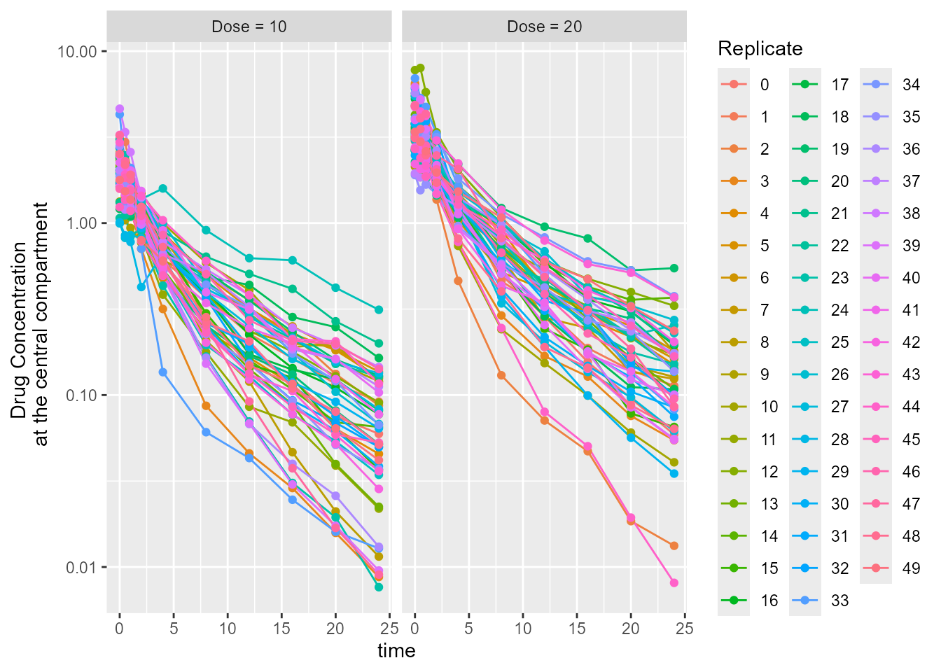

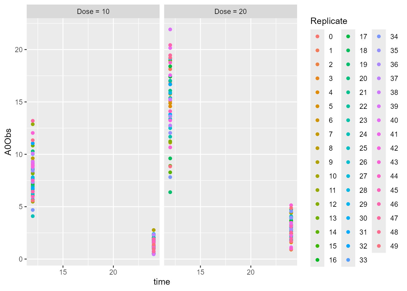
  ## Simulated urine observations 
  dt_A0Obs <- job$SimTableA0Obs
  setnames(dt_A0Obs, c("# repl"), c("Replicate"))
  dt_A0Obs$Replicate <- as.factor(dt_A0Obs$Replicate)
  dt_A0Obs$id5 <- as.factor(dt_A0Obs$id5)
  levels(dt_A0Obs$id5) = c(paste0("Dose = ", dt_SimInputData$Dose[1]),
                           paste0("Dose = ", dt_SimInputData$Dose[2]))

  ## Plot simulated urine observations
  ggplot(dt_A0Obs, aes(x = time, y = A0Obs, group = Replicate, color = Replicate)) + 
    geom_point() +
    facet_grid(.~ id5)