Models with Categorical Data
categorical_data.Rmd
Overview
The purpose of this vignette is to demonstrate how to: * Fit a model
defined by PML codes, where + the PK portion of the model is described
by a one-compartment model with first-order absorption + the PD portion
of the model is described by an Emax model and a categorical model with
three categories * Import estimation results to xpose database to create
some commonly used diagnostic plots for each continuous observed
variable * Perform VPC for the model * Create VPC plots through open
source package tidyvpc (command-line usage) and VPC results
Shiny app (in Certara.VPCResults package) We assume that
all the necessary packages are loaded and the directory with NLME
Executables is given as an environment variable
(INSTALLDIR).
# loading the package
library(Certara.RsNLME)
library(data.table)
library(dplyr)
library(xpose)
library(Certara.Xpose.NLME)
library(ggplot2)
library(Certara.ModelResults)
library(Certara.VPCResults)
library(tidyvpc)

# Check the environment variable
Sys.getenv("INSTALLDIR")
Create the textual model
We will use the data
OneCpt1stOrderAbsorp_Emax_CategoricalModel.csv and the PML
model file OneCpt1stOrderAbsorp_Emax_CategoricalModel.mdl
distributed with the Certara.RsNLME package. First, we will
import the data
filename <- system.file("vignettesdata/OneCpt1stOrderAbsorp_Emax_CategoricalModel.csv",
                        package = "Certara.RsNLME",
                        mustWork = TRUE)
dt_InputDataSet <- fread(filename)
Next we will locate the PML model file and then create a textual model object for it.
filename <- system.file("vignettesdata/OneCpt1stOrderAbsorp_Emax_CategoricalModel.mdl",
                        package = "Certara.RsNLME",
                        mustWork = TRUE)

# Load the PML codes and link it to associated input data to create a model object
model <- textualmodel(modelName = "OneCpt1stOrderAbsorp_Emax_CategoricalModel",
                      mdl = filename,
                      data = dt_InputDataSet)
Let’s view the model and its associated column mappings, and then map those un-mapped model variables to their corresponding input data columns:
# View the model and its associated column mappings
print(model)

 Model Overview
 -------------------------------------------
Model Name        :  OneCpt1stOrderAbsorp_Emax_CategoricalModel
Working Directory :  /TestEnvironment/
Model Type        :  Textual

 PML
 -------------------------------------------
test(){

    # ===============================================================
    # PK model: one compartment model with 1st order absorption
    # ===============================================================
    cfMicro(A1, Cl / V, first = (Aa = Ka))
    dosepoint(Aa)
    C = A1 / V

    # residual error model
    error(CEps = 0.1)
    observe(CObs = C * (1 + CEps))

    # ----------------------------------------------------------------
    # PK model parameters
    # ----------------------------------------------------------------
    # Structural model parameters
    stparm(Ka = exp(tvlogKa + nlogKa))
    stparm(V = exp(tvlogV + nlogV))
    stparm(Cl = exp(tvlogCl + nlogCl))

    # fixed effects
    fixef(tvlogKa = c(, -1, ))
    fixef(tvlogV = c(, 2, ))
    fixef(tvlogCl = c(, 0, ))

    # random effects
    ranef(diag(nlogV, nlogCl, nlogKa) = c(1, 1, 1))


    # ================================================================
    # PD model
    # ================================================================
    E = Emax * C / (EC50 + C)

    ## Residual error model
    error(EEps = 0.1)
    observe(EObs = E * (1 + EEps))

    ## Categorical model
    multi(CategoricalObs, ilogit, -E, -(E + CatParam))

    # ----------------------------------------------------------------
    # Categorical model parameters
    # ----------------------------------------------------------------
    # structural model parameters
    stparm(EC50 = exp(tvlogEC50 + nlogEC50))
    stparm(Emax = exp(tvlogEmax + nlogEmax))
    stparm(CatParam = exp(tvlogCatParam + nlogCatParam))

    # fixed effects
    fixef(tvlogEC50 = c(, 2, ))
    fixef(tvlogEmax = c(, -2, ))
    fixef(tvlogCatParam = c(, 1, ))

    # random effects
    ranef(diag(nlogEC50, nlogEmax, nlogCatParam) = c(1, 1, 1))
}

 Structural Parameters
 -------------------------------------------
 Ka V Cl EC50 Emax CatParam
 -------------------------------------------
 Column Mappings
 -------------------------------------------
Model Variable Name : Data Column name
id                  : ?
time                : time
Aa                  : ?
CObs                : CObs
EObs                : EObs
CategoricalObs      : CategoricalObs

# Manually map those un-mapped model variables to their corresponding input data columns
model <- model %>%
  colMapping(c(id = "SubID", Aa = "dose_Aa"))
Model Fitting
Next, we will run the model using the fitmodel
function with default host. We will use the QRPEM method for fitting. We
will also output residuals PCWRES with the number of replicates set to
be 1000 (Note: PCWRES is not outputted by default).
job <- fitmodel(model, method = "QRPEM", numRepPCWRES = 1000)Diagnostic Plots
We will use the xposeNlme
function from the Certara.Xpose.NLME package to import
estimation results to xpose database to create some
commonly used diagnostic plots. All the functions provided in the
xpose package can be used. Here we only demonstrate several
of these functions.
## Imports results of an NLME run into xpose database to create commonly used diagnostic plots
xp <- xposeNlme(dir = model@modelInfo@workingDir,
                modelName = "OneCpt1stOrderAbsorp_Emax_CategoricalModel")

## Filter out CategoricalObs
xp <- xp %>%
  filter(ObsName != "CategoricalObs")

## observations against population predictions
dv_vs_pred(xp,
           type = "p",
           facets = "ObsName",
           subtitle = "-2LL: @ofv",
           caption = "dv_vs_pred")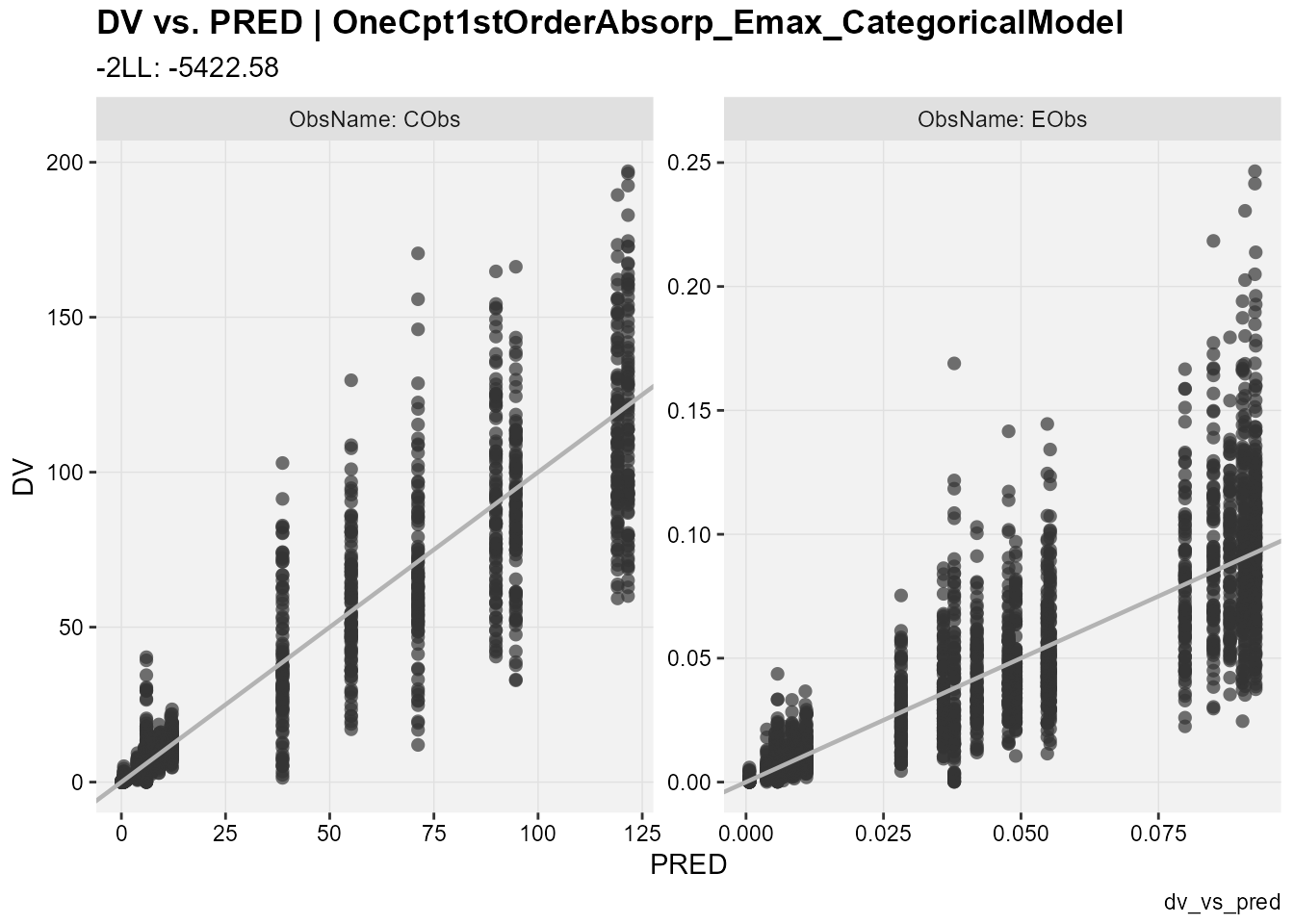
## observations against individual predictions
dv_vs_ipred(xp,
            type = "p",
            facets = "ObsName",
            subtitle = "-2LL: @ofv, Eps shrinkage: @epsshk",
            caption = "dv_vs_ipred")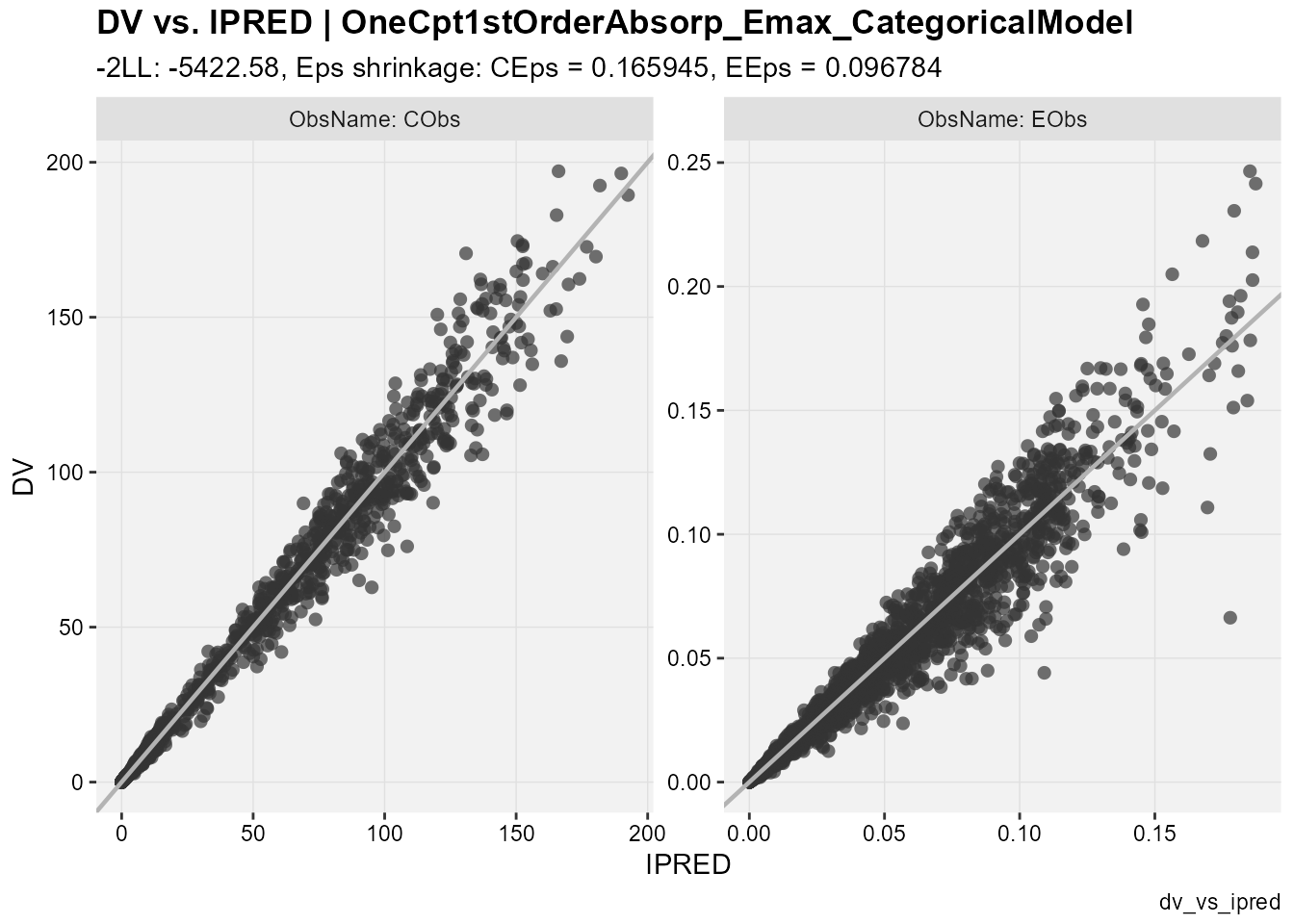
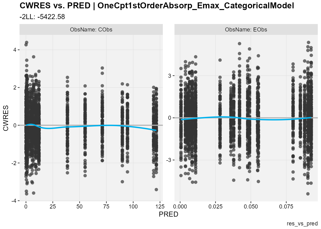
## CWRES against population predictions
res_vs_pred(
  xp,
  res = "CWRES",
  type = "ps",
  facets = "ObsName",
  subtitle = "-2LL: @ofv",
  caption = "res_vs_pred"
)
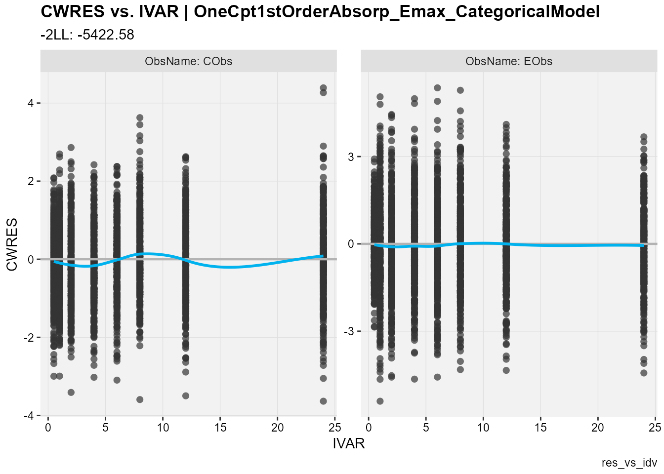
## CWRES against the independent variable
res_vs_idv(
  xp,
  res = "CWRES",
  type = "ps",
  facets = "ObsName",
  subtitle = "-2LL: @ofv",
  caption = "res_vs_idv"
)
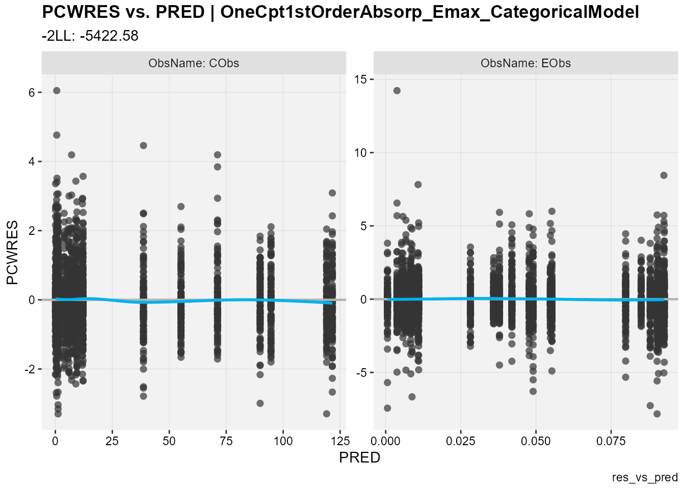
## PCWRES against population predictions
res_vs_pred(
  xp,
  res = "PCWRES",
  type = "ps",
  facets = "ObsName",
  subtitle = "-2LL: @ofv",
  caption = "res_vs_pred"
)
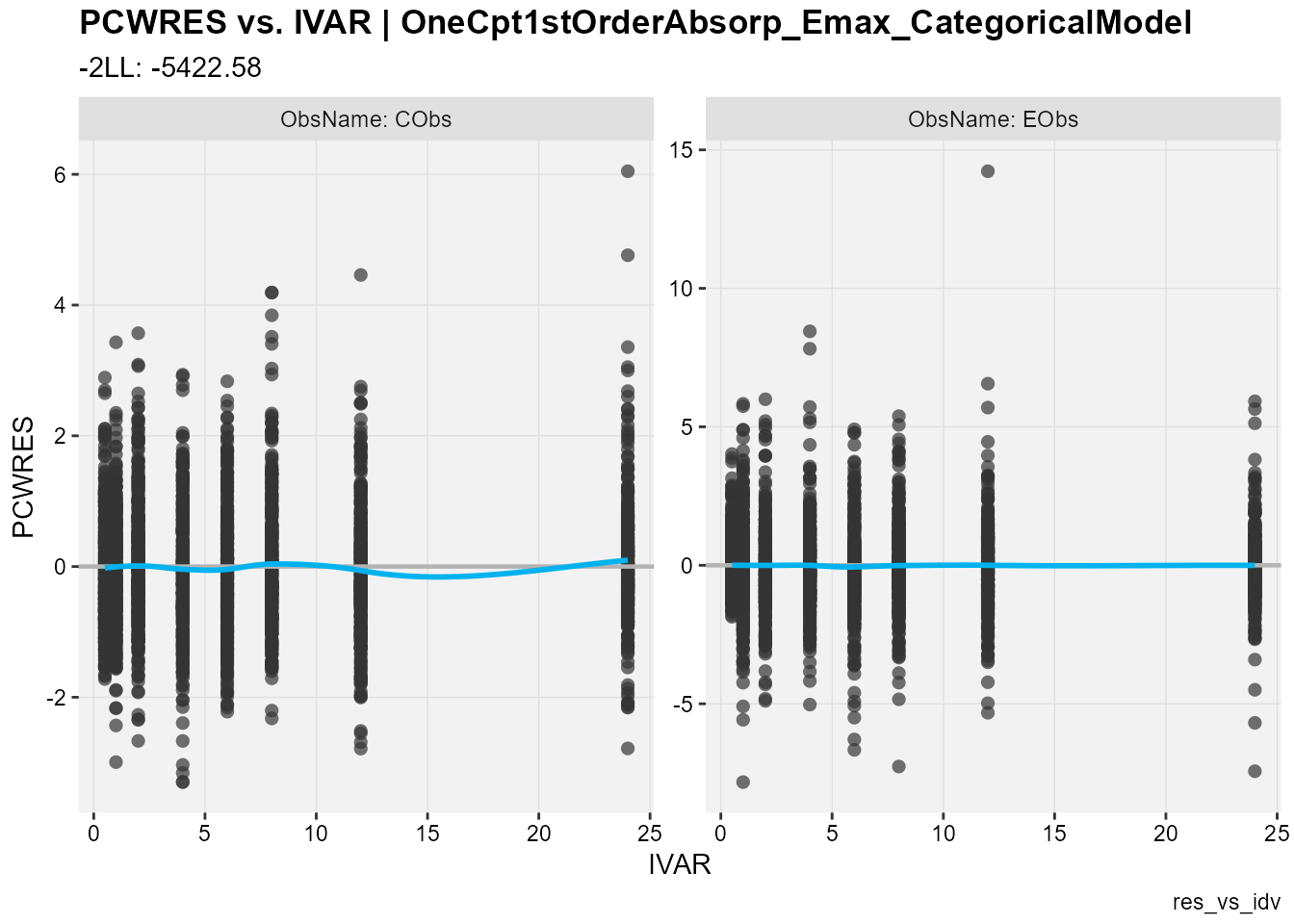
## PCWRES against the independent variable
res_vs_idv(
  xp,
  res = "PCWRES",
  type = "ps",
  facets = "ObsName",
  subtitle = "-2LL: @ofv",
  caption = "res_vs_idv"
)
Alternatively, one can view/customize diagnostic plots as well as
estimation results using the Certara.ModelResults Shiny
application, which can also be used to generate .R and/or
.Rmd code based on operations performed in the GUI. For
installation and usage details, please visit the following link.
Here we only demonstrate how to invoke this Shiny app through either the
NlmePmlModel object or the xpose_data object
created above.
library(Certara.ModelResults)
## Invoke model results shiny app through model object defined above
resultsUI(model = model)

## Alternatively, one can invoke model results shiny app through xpose data object created above
resultsUI(xpdb = xp)
VPC
We will use the copyModel
function to copy the model into a new object and accept final parameter
estimates from fitting run as initial estimates for VPC simulation:
modelVPC <- copyModel(model,
                      acceptAllEffects = TRUE,
                      modelName = "OneCpt1stOrderAbsorp_Emax_CategoricalModel_VPC")
## View model
print(modelVPC)
Model Overview
-------------------------------------------
Model Name : OneCpt1stOrderAbsorp_Emax_CategoricalModel_VPC
Working Directory : /TestEnvironment/
Model Type : Textual
PML
-------------------------------------------
test(){
# ===============================================================
# PK model: one compartment model with 1st order absorption
# ===============================================================
cfMicro(A1, Cl / V, first = (Aa = Ka))
dosepoint(Aa)
C = A1 / V
# residual error model
error(CEps = 0.121544989390655)
observe(CObs = C * (1 + CEps))
# ----------------------------------------------------------------
# PK model parameters
# ----------------------------------------------------------------
# Structural model parameters
stparm(Ka = exp(tvlogKa + nlogKa))
stparm(V = exp(tvlogV + nlogV))
stparm(Cl = exp(tvlogCl + nlogCl))
# fixed effects
fixef(tvlogKa = c(,-0.356862376105887,))
fixef(tvlogV = c(,1.63701201332346,))
fixef(tvlogCl = c(,-0.224407387665085,))
# random effects
ranef(diag(nlogV, nlogCl, nlogKa) = c(0.086623473, 0.1052053, 0.11503702))
# ================================================================
# PD model
# ================================================================
E = Emax * C / (EC50 + C)
## Residual error model
error(EEps = 0.179381191063015)
observe(EObs = E * (1 + EEps))
## Categorical model
multi(CategoricalObs, ilogit, -E, -(E + CatParam))
# ----------------------------------------------------------------
# Categorical model parameters
# ----------------------------------------------------------------
# structural model parameters
stparm(EC50 = exp(tvlogEC50 + nlogEC50))
stparm(Emax = exp(tvlogEmax + nlogEmax))
stparm(CatParam = exp(tvlogCatParam + nlogCatParam))
# fixed effects
fixef(tvlogEC50 = c(,2.28995796141293,))
fixef(tvlogEmax = c(,-2.30045875119332,))
fixef(tvlogCatParam = c(,0.418715524585389,))
# random effects
ranef(diag(nlogEC50, nlogEmax, nlogCatParam) = c(0.066093482, 0.10266479, 0.15212821))
}
Structural Parameters
-------------------------------------------
Ka V Cl EC50 Emax CatParam
-------------------------------------------
Column Mappings
-------------------------------------------
Model Variable Name : Data Column name
id : SubID
time : time
Aa : dose_Aa
CObs : CObs
EObs : EObs
CategoricalObs : CategoricalObsNow, let’s run VPC using the vpcmodel
function with the default host, default values for the relevant NLME
engine arguments, and PRED outputted.
Note: Here we define VPC argument, outputPRED,
through ellipsis (additional argument). Alternatively, one can define
VPC arguments through vpcParams
argument.
vpcJob <- vpcmodel(modelVPC, outputPRED = TRUE)

## predcheck0 contains observed data for all continuous observed variables
dt_ObsData_ContinuousObs <- vpcJob$predcheck0

## predcheck0_cat contains observed data for Categorical/count observed variables
dt_ObsData_CategoricalObs <- vpcJob$predcheck0_cat

## predout contains simulated data for all observed variables
dt_SimData <- vpcJob$predout
Next we will create VPC plots through tidyvpc package.
The tidyvpc package provides support for both continuous
and categorical VPC using both binning and binless methods. For details
on this package, please visit the following link. Note that
this example contains 3 observed variable with PRED outputted. Hence, to
use this package, we have to do some data preprocessing on both
simulated and observed data to meet the requirements set by the
tidyvpc package.
First we will process the simulated data output to pass to the
simulated() function in the tidyvpc package,
creating a separate data.frame for each of our
DV:
## Extract simulated data for observed variable "CObs"
dt_SimData_tidyvpc_CObs <- dt_SimData[OBSNAME == "CObs"]
## Extract simulated data for observed variable "EObs"
dt_SimData_tidyvpc_EObs <- dt_SimData[OBSNAME == "EObs"]
## Extract simulated data for observed variable "CategoricalObs"
dt_SimData_tidyvpc_CategoricalObs <- dt_SimData[OBSNAME == "CategoricalObs"]
Next, we will process the observed data output to pass to the
observed() function in the tidyvpc package,
creating a separate data.frame for each of our
DV as we did for the simulated data output:
## Extract observed data for observed variable "CObs"
dt_ObsData_ContinuousObs_tidyvpc_CObs <- dt_ObsData_ContinuousObs[ObsName == "CObs"]
## Extract observed data for observed variable "EObs"
dt_ObsData_ContinuousObs_tidyvpc_EObs <- dt_ObsData_ContinuousObs[ObsName == "EObs"]
## Extract observed data for observed variable "CategoricalObs"
dt_ObsData_CategoricalObs_tidyvpc <- dt_ObsData_CategoricalObs[ObsName == "CategoricalObs"]
Finally, we will add the $PRED column from
REPLICATE == 0 ($PRED may be extracted from
any REPLICATE) in the simulated data to our observed data
in order to perform a prediction-corrected VPC:
## Add PRED from REPLICATE == 0 of simulated data (CObs) to observed data (CObs)
dt_ObsData_ContinuousObs_tidyvpc_CObs$PRED <- as.numeric(dt_SimData_tidyvpc_CObs[REPLICATE == 0]$PRED)

## Add PRED from REPLICATE == 0 of simulated data (EObs) to observed data (EObs)
dt_ObsData_ContinuousObs_tidyvpc_EObs$PRED <- as.numeric(dt_SimData_tidyvpc_EObs[REPLICATE == 0]$PRED)
Now we can create VPC plots.
### Create a binless VPC plot for CObs
binless_VPC_CObs <- observed(dt_ObsData_ContinuousObs_tidyvpc_CObs, x = IVAR, yobs = DV) %>%
  simulated(dt_SimData_tidyvpc_CObs, ysim = DV) %>%
  binless() %>%
  vpcstats()
plot(binless_VPC_CObs)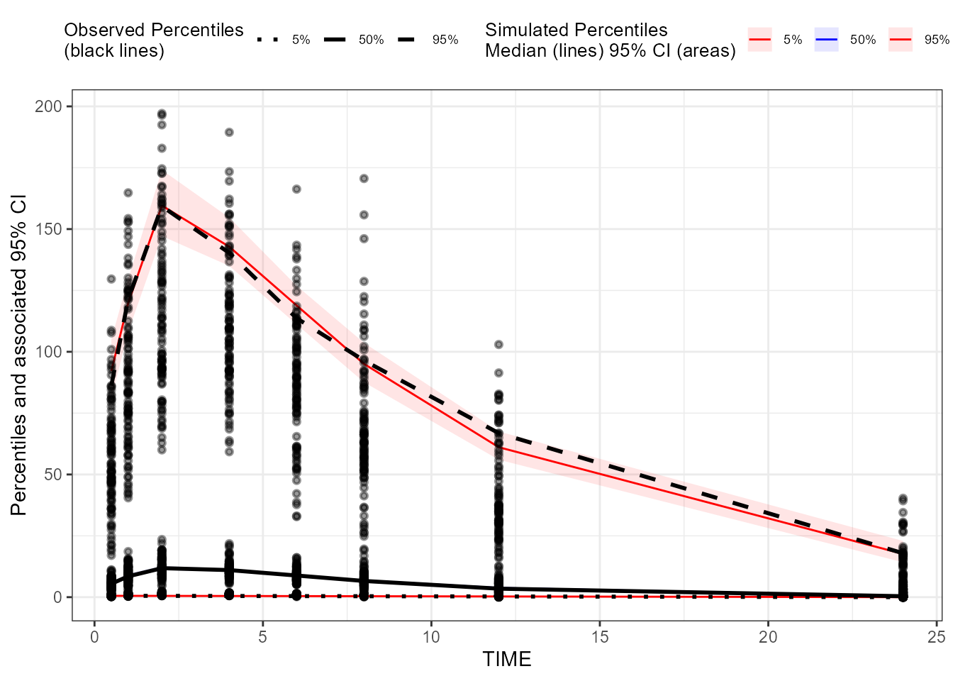
### Create a binless pcVPC plot for CObs
binless_pcVPC_CObs <- observed(dt_ObsData_ContinuousObs_tidyvpc_CObs,
                               x = IVAR,
                               yobs = DV) %>%
  simulated(dt_SimData_tidyvpc_CObs, ysim = DV) %>%
  binless(loess.ypc = TRUE) %>%
  predcorrect(pred = PRED) %>%
  vpcstats()
plot(binless_pcVPC_CObs)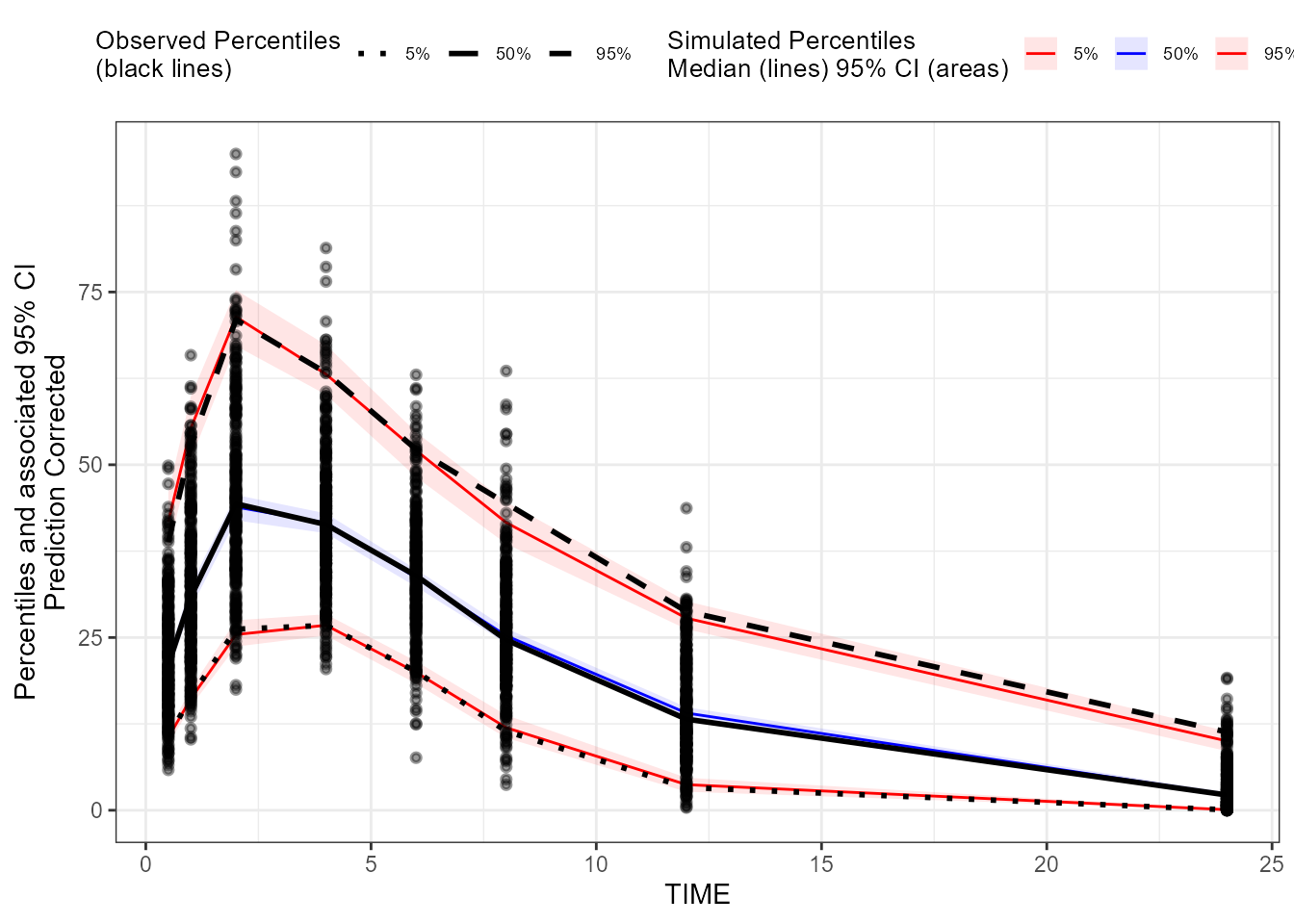
### Create a binless VPC plot for EObs
binless_VPC_EObs <- observed(dt_ObsData_ContinuousObs_tidyvpc_EObs, x = IVAR, yobs = DV) %>%
  simulated(dt_SimData_tidyvpc_EObs, ysim = DV) %>%
  binless() %>%
  vpcstats()
plot(binless_VPC_EObs)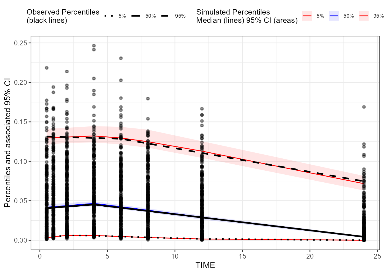
### Create a binless pcVPC plot for EObs
binless_pcVPC_EObs <- observed(dt_ObsData_ContinuousObs_tidyvpc_EObs, x = IVAR, yobs = DV) %>%
  simulated(dt_SimData_tidyvpc_EObs, ysim = DV) %>%
  binless(loess.ypc = TRUE) %>%
  predcorrect(pred = PRED) %>%
  vpcstats()
plot(binless_pcVPC_EObs)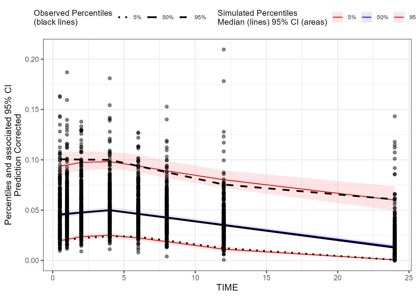
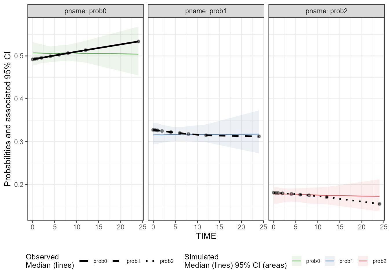
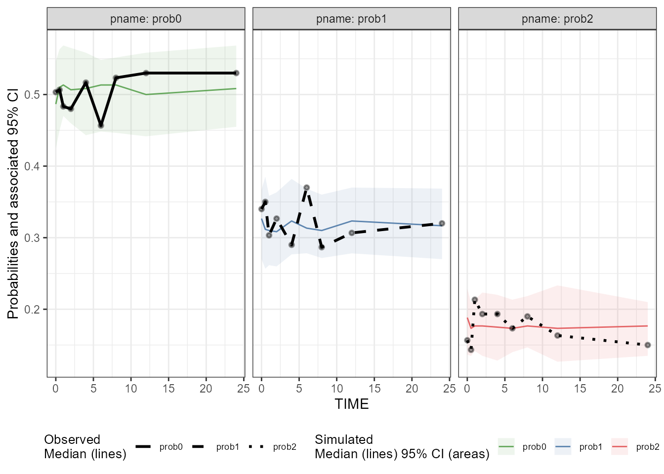
### Create a binless VPC plot for CatgoricalObs
binless_VPC_CategoricalObs <- observed(dt_ObsData_CategoricalObs_tidyvpc,
                                       x = IVAR,
                                       yobs = DV) %>%
  simulated(dt_SimData_tidyvpc_CategoricalObs, ysim = DV) %>%
  binless() %>%
  vpcstats(vpc.type = "categorical")

plot(binless_VPC_CategoricalObs
     , facet = TRUE
     , facet.scales = "fixed"
     , legend.position = "bottom"
    )
### Create a binning VPC plot for CObs: binning on x-variable itself
binning_VPC_CObs <- observed(dt_ObsData_ContinuousObs_tidyvpc_CObs, x = IVAR, yobs = DV) %>%
  simulated(dt_SimData_tidyvpc_CObs, ysim = DV) %>%
  binning(bin = IVAR) %>%
  vpcstats()
plot(binning_VPC_CObs)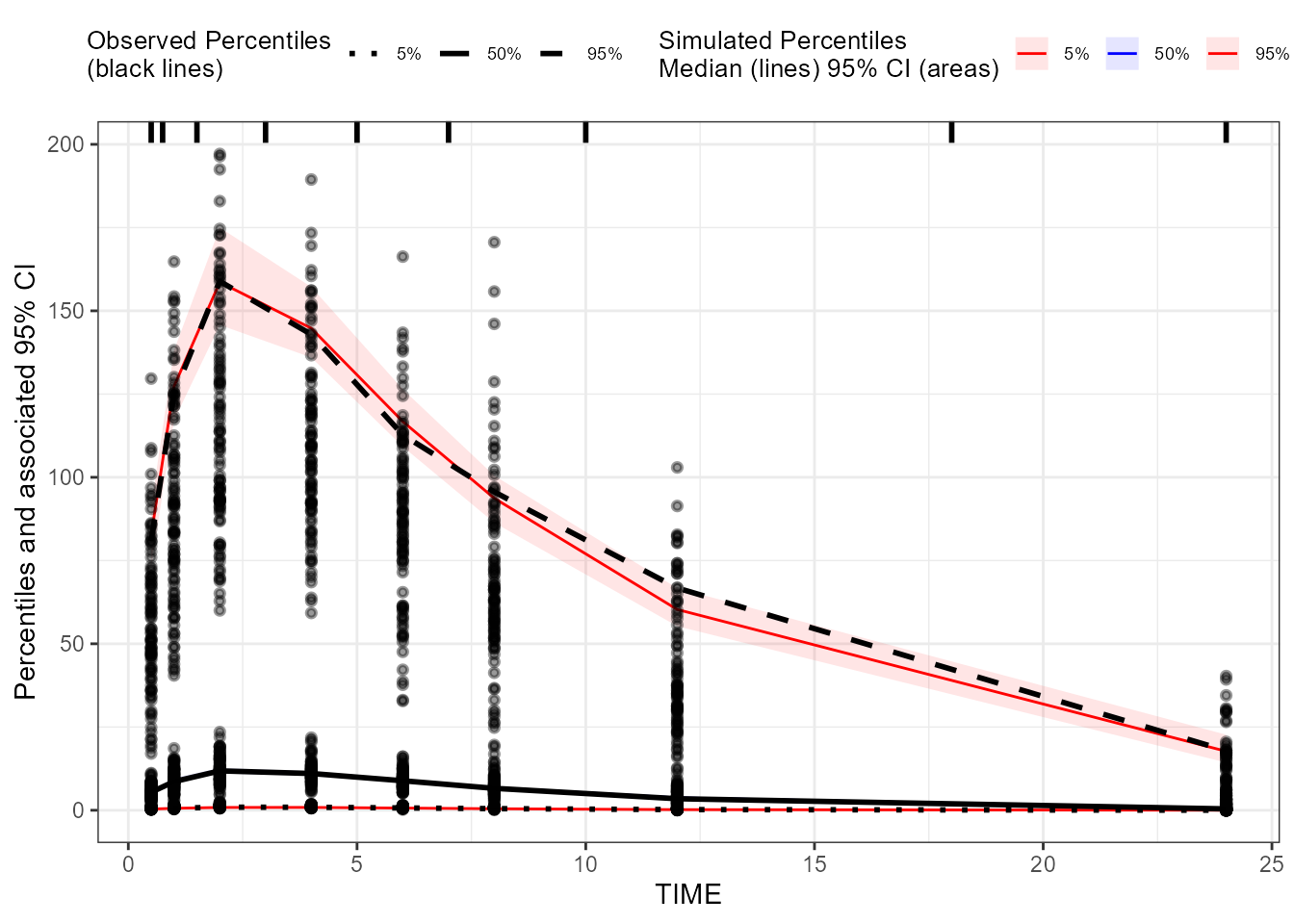
### Create a binning pcVPC plot for CObs: binning on x-variable itself
binning_pcVPC_CObs <- observed(dt_ObsData_ContinuousObs_tidyvpc_CObs,
                               x = IVAR,
                               yobs = DV) %>%
  simulated(dt_SimData_tidyvpc_CObs, ysim = DV) %>%
  binning(bin = IVAR) %>%
  predcorrect(pred = PRED) %>%
  vpcstats()
plot(binning_pcVPC_CObs)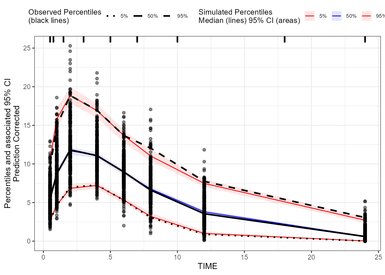
### Create a binning VPC plot for EObs: binning on x-variable itself
binning_VPC_EObs <- observed(dt_ObsData_ContinuousObs_tidyvpc_EObs, x = IVAR, yobs = DV) %>%
  simulated(dt_SimData_tidyvpc_EObs, ysim = DV) %>%
  binning(bin = IVAR) %>%
  vpcstats()
plot(binning_VPC_EObs)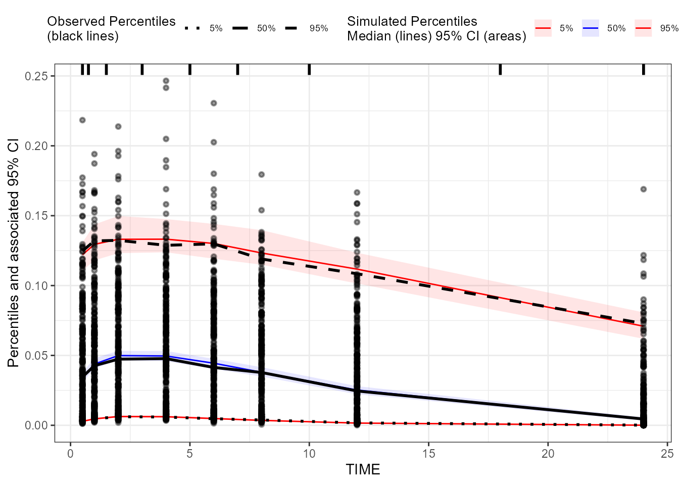
### Create a binning pcVPC plot for EObs: binning on x-variable itself
binning_pcVPC_EObs <- observed(dt_ObsData_ContinuousObs_tidyvpc_EObs, x = IVAR, yobs = DV) %>%
  simulated(dt_SimData_tidyvpc_EObs, ysim = DV) %>%
  binning(bin = IVAR) %>%
  predcorrect(pred = PRED) %>%
  vpcstats()
plot(binning_pcVPC_EObs)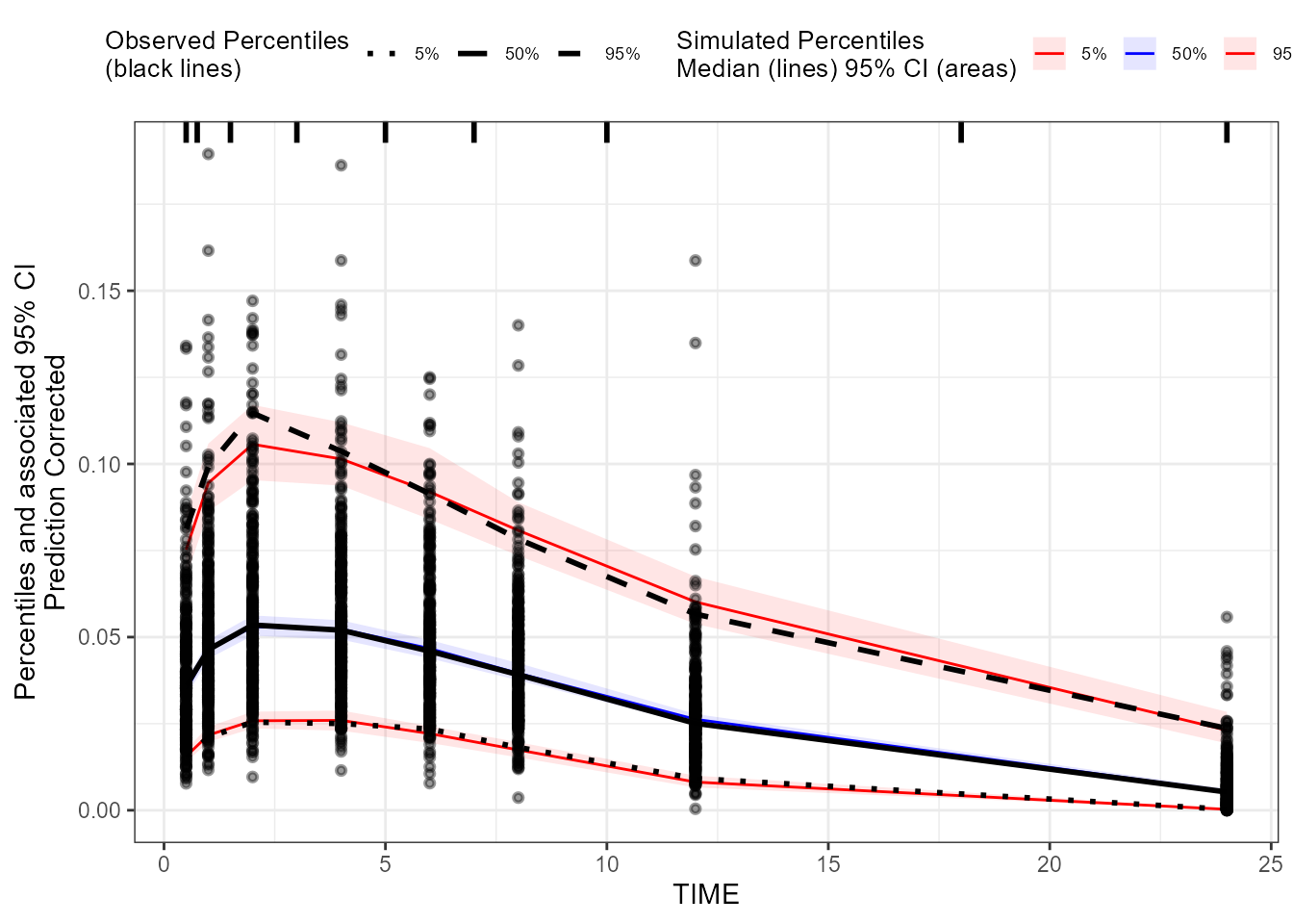
### Create a binning VPC plot for CatgoricalObs: binning on x-variable itself
binning_VPC_CategoricalObs <- observed(dt_ObsData_CategoricalObs_tidyvpc,
                                       x = IVAR,
                                       yobs = DV) %>%
  simulated(dt_SimData_tidyvpc_CategoricalObs, ysim = DV) %>%
  binning(bin = IVAR) %>%
  vpcstats(vpc.type = "categorical")

plot(binning_VPC_CategoricalObs
     , facet = TRUE
     , facet.scales = "fixed"
     , legend.position = "bottom"
    )
Alternatively, one can create/customize VPC plots through VPC results
shiny app (in Certara.VPCResults package), which can also
be used to:
- generate corresponding tidyvpc code to reproduce the VPC ouput from R command line
- generate report as well as the associated R markdown.
Here we only demonstrate how to invoke this shiny app (Note: The shiny app will automatically preprocess the data as what we did above for tidyvpc package).
library(Certara.VPCResults)
## Invoke VPC results shiny app to create VPC plots for CObs
taggedVPC_CObs <- vpcResultsUI(observed = dt_ObsData_ContinuousObs_tidyvpc_CObs,
                               simulated = dt_SimData_tidyvpc_CObs)

## Invoke VPC results shiny app to create VPC plots for EObs
taggedVPC_EObs <- vpcResultsUI(observed = dt_ObsData_ContinuousObs_tidyvpc_EObs,
                               simulated = dt_SimData_tidyvpc_EObs)

## Invoke VPC results shiny app to create  VPC plot for categoricalObs
taggedVPC_CategoricalObs <- vpcResultsUI(observed = dt_ObsData_CategoricalObs_tidyvpc,
                                         simulated = dt_SimData_tidyvpc_CategoricalObs,
                                         vpc.type = "categorical")