ETAs vs covariate Plot
eta_vs_cov.RdPlot ETAs against a continuous or categorical covariate.
Usage
eta_vs_cov(
  xpdb,
  covariate,
  mapping = NULL,
  drop_fixed = FALSE,
  group = "ID",
  type = "bpls",
  title = "ETAs vs @x | @run",
  subtitle = "Based on @nind individuals",
  caption = "@dir",
  tag = NULL,
  log = NULL,
  guide = FALSE,
  onlyfirst = TRUE,
  facets,
  .problem,
  quiet,
  ...
)
Arguments
- xpdb
An xpose database object.
- covariate
Character; String of covariate name
- mapping
List of aesthetics mappings to be used for the xpose plot (e.g.
point_color).- drop_fixed
Logical; Logic specifying whether ETAs having same value for the given covariate value should be removed from plotting
- group
Grouping variable to be used for lines.
IDby default- type
Character; String setting the type of plot to be used. Must be 'b' for categorical covariates, one or a combination of 'p','l','s' for continuous covariates.
- title
Character; Plot title. Use
NULLto remove.- subtitle
Character; Plot subtitle. Use
NULLto remove.- caption
Character; Page caption. Use
NULLto remove.- tag
Character; Plot identification tag. Use
NULLto remove.- log
Character; String assigning logarithmic scale to axes, can be either ”, 'x', y' or 'xy'.
- guide
Logical; Should the guide (e.g. reference distribution) be displayed.
- onlyfirst
Logical; Should the data be filtered to retain first value for each group/facet.
- facets
Either a character string to use
facet_wrap_paginateor a formula to usefacet_grid_paginate.- .problem
The $problem number to be used. By default returns the last estimation problem.
- quiet
Logical, if
FALSEmessages are printed to the console.- ...
Any additional aesthetics to be passed on
xplot_scatterorxplot_box.
Value
An object of class xpose_plot, ggplot, and gg. This object represents a customized plot created using ggplot2.
The xpose_plot class provides additional metadata and integration with xpose workflows, allowing for advanced
customization and compatibility with other xpose functions. Users can interact with the plot object as they
would with any ggplot2 object, including modifying aesthetics, adding layers, or saving the plot.
Layers mapping
Plots can be customized by mapping arguments to specific layers. The naming convention is layer_option where layer is one of the names defined in the list below and option is any option supported by this layer e.g. boxplot_fill = 'blue', etc.
box plot: options to
geom_boxplotpoint plot: options to
geom_pointline plot: options to
geom_linesmooth plot: options to
geom_smoothxscale: options to
scale_x_continuousorscale_x_log10yscale: options to
scale_y_continuousorscale_y_log10
Examples
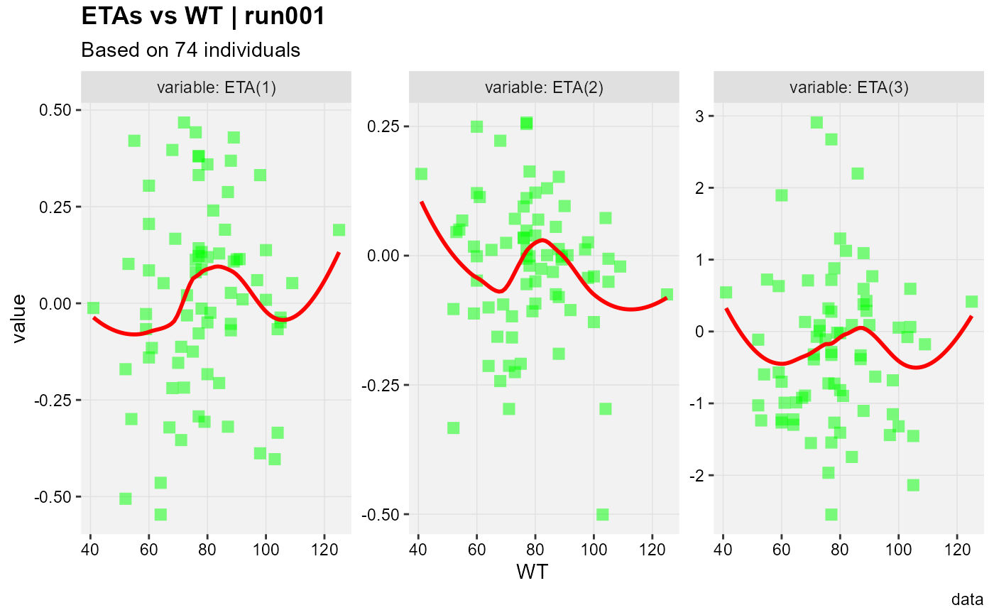
eta_vs_cov(xpose::xpdb_ex_pk,
covariate = "WT",
type = "ps",
smooth_color = "red",
point_color = "green",
point_shape = "square",
point_alpha = .5,
point_size = 3
)
#> Using data from $prob no.1
#> Removing duplicated rows based on: ID
#> Tidying data by ID, SEX, MED1, MED2, DOSE ... and 23 more variables
#> `geom_smooth()` using formula = 'y ~ x'
#> `geom_smooth()` using formula = 'y ~ x'
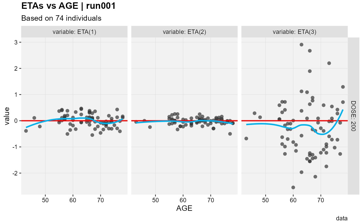
 eta_vs_cov(xpose::xpdb_ex_pk,
covariate = "AGE",
type = "ps",
facets = DOSE ~ variable,
guide = TRUE,
guide_color = "red",
guide_slope = 0,
guide_intercept = 0
)
#> Using data from $prob no.1
#> Removing duplicated rows based on: ID, DOSE
#> Tidying data by ID, SEX, MED1, MED2, DOSE ... and 23 more variables
#> `geom_smooth()` using formula = 'y ~ x'
#> `geom_smooth()` using formula = 'y ~ x'
eta_vs_cov(xpose::xpdb_ex_pk,
covariate = "AGE",
type = "ps",
facets = DOSE ~ variable,
guide = TRUE,
guide_color = "red",
guide_slope = 0,
guide_intercept = 0
)
#> Using data from $prob no.1
#> Removing duplicated rows based on: ID, DOSE
#> Tidying data by ID, SEX, MED1, MED2, DOSE ... and 23 more variables
#> `geom_smooth()` using formula = 'y ~ x'
#> `geom_smooth()` using formula = 'y ~ x'