Exploring Model Diagnostics
exploring_model_diagnostics.RmdThe purpose of this vignette is to demonstrate how to:
- Create an
xpose_dataobject from NLME model execution directory/files - Utilize functions from the
xposepackage to generate basic GOF plots - Extend
xposeplot functions withggplot2 - Explore application of covariate model diagnostics functions, only
available in
Certara.Xpose.NLME - Extract GOF data from the
xpose_dataobject and explore usage ofggcertara
Note: The corresponding R script used in this example can be
found in
RsNLME_Examples/TwoCptIVBolus_FitBaseModel_CovariateSearch_VPC_BootStrapping.R.
See RsNLME
Example Scripts.
Data
We will be using the built-in pkData from the
Certara.RsNLME package for the following examples.
pkData is a pharmacokinetic dataset containing 16 subjects
with single bolus dose.
library(Certara.RsNLME)
library(dplyr)
library(magrittr)

pkData <- Certara.RsNLME::pkData

glimpse(pkData)
#> Rows: 112
#> Columns: 8
#> $ Subject    <dbl> 1, 1, 1, 1, 1, 1, 1, 2, 2, 2, 2, 2, 2, 2, 3, 3, 3, 3, 3, 3,…
#> $ Nom_Time   <dbl> 0, 1, 1, 2, 4, 8, 24, 0, 1, 1, 2, 4, 8, 24, 0, 1, 1, 2, 4, …
#> $ Act_Time   <dbl> 0.00, 0.26, 1.10, 2.10, 4.13, 8.17, 23.78, 0.00, 0.37, 0.83…
#> $ Amount     <dbl> 25000, NA, NA, NA, NA, NA, NA, 25000, NA, NA, NA, NA, NA, N…
#> $ Conc       <dbl> 2010.0, 1330.0, 565.0, 216.0, 180.0, 120.0, 16.9, 850.0, 79…
#> $ Age        <dbl> 22, 22, 22, 22, 22, 22, 22, 46, 46, 46, 46, 46, 46, 46, 52,…
#> $ BodyWeight <dbl> 73, 73, 73, 73, 73, 73, 73, 79, 79, 79, 79, 79, 79, 79, 63,…
#> $ Gender     <chr> "male", "male", "male", "male", "male", "male", "male", "fe…
Model Building and Execution
Before exploring usage of Certara.Xpose.NLME and
evaulating our covariate model diagnostic functions, we will first:
- Build and execute our base model
- Copy the base model and accept parameter estimates
- Add continuous and categorical covariates to the new model
- Execute the new covariate model
For a detailed explanation on model building and execution in
Certara.RsNLME visit here.
Build and execute base model
# Create model
baseModel <- pkmodel(
  numCompartments = 2, data = pkData,
  ID = "Subject", Time = "Act_Time", A1 = "Amount", CObs = "Conc",
  modelName = "TwCpt_IVBolus_FOCE_ELS"
)

# Update parameters
baseModel <- baseModel %>%
  structuralParameter(paramName = "V2", hasRandomEffect = FALSE) %>%
  fixedEffect(effect = c("tvV", "tvCl", "tvV2", "tvCl2"), value = c(15, 5, 40, 15)) %>%
  randomEffect(effect = c("nV", "nCl", "nCl2"), value = rep(0.1, 3)) %>%
  residualError(predName = "C", SD = 0.2)

# Fit model
baseFitJob <- fitmodel(baseModel)
Copy model and accept parameter estimates
covariateModel <- copyModel(baseModel,
  acceptAllEffects = TRUE,
  modelName = "TwCpt_IVBolus_SelectedCovariateModel_FOCE_ELS"
)
Add covariates to new model and fit
covariateModel <- covariateModel %>%
  addCovariate(covariate = c(Sex = "Gender"), effect = c("V", "Cl"), type = "Categorical", levels = c(0, 1), labels = c("female", "male")) %>%
  addCovariate(covariate = "Age", effect = c("V", "Cl")) %>%
  addCovariate(covariate = c(BW = "BodyWeight"), effect = c("V", "Cl"), center = "Value", centerValue = 70)


covariateJob <- fitmodel(covariateModel)
Create xpose_data object from RsNLME model output
We can create our xpose_data object from our RsNLME
output by supplying the output directory where our model execution files
have been saved. If the model in your R environment has been executed
previously, you may pass the folder path from
model@modelInfo@workingDir directly to the dir
argument of the xposeNlme() function.
library(Certara.Xpose.NLME)
library(xpose)

xpdb <- xposeNlme(dir = covariateModel@modelInfo@workingDir)

class(xpdb)
#> [1] "xpose_data" "uneval"
List available variables
We will use the list_vars() function from
xpose to print out useful information about our
xpose_data object.
list_vars(xpdb)
#>
#> List of available variables for problem no. 1
#>  - Subject identifier (id)               : ID
#>  - Dependent variable (dv)               : DV
#>  - Independent variable (idv)            : IVAR
#>  - DV identifier (dvid)                  : ObsName
#>  - Dose amount (amt)                     : Amount
#>  - Event identifier (evid)               : EVID
#>  - Model typical predictions (pred)      : PRED
#>  - Model individual predictions (ipred)  : IPRED
#>  - Model parameter (param)               : V, Cl, V2, Cl2
#>  - Eta (eta)                             : nV, nCl, nCl2
#>  - Residuals (res)                       : IRES, IWRES, WRES, CWRES
#>  - Categorical covariates (catcov)       : Sex
#>  - Continuous covariates (contcov)       : Age, BW
#>  - Not attributed (na)                   : Subject, Nom_Time, Act_Time, Conc, BodyWeight, Gender, WhichReset, TIME, TAD, PREDSE, Weight, WhichDose
Covariate Model Diagnostics
Covariate model diagnostics plot types vary given the covariate type (continuous or categorical). Continuous covariates are plotted in a scatter plot, while categorical covariates in a box plot.
The following “xpose-like” covariate model diagnostics functions are
available in Certara.Xpose.Nlme:
- res_vs_cov()
- prm_vs_cov()
- eta_vs_cov()
The above functions follow xpose conventions, including
usage of the type argument to specify the type of plot
attributes and usage of the ... ellipses to allow pass
through geom arguments from ggplot2.
Note: The returned plot from xpose and
Certara.Xpose.Nlme is of class ggplot,
therefore functions from ggplot2 can be applied to the plot
for further customized styling.
Residuals vs Covariate
Let’s look inside the data and preview which residuals are available for plotting.
library(dplyr)
library(xpose)

gofData <- get_data(xpdb)

gofData %>%
  select(ends_with("RES"))
#> # A tibble: 112 × 4
#>       IRES  IWRES   WRES  CWRES
#>      <dbl>  <dbl>  <dbl>  <dbl>
#>  1  260.    0.937  1.16   1.12
#>  2  119.    0.618  0.666  0.645
#>  3  110.    1.52   1.09   1.08
#>  4  -24.0  -0.629 -1.01  -1.07
#>  5   19.7   0.774  0.488  0.545
#>  6   14.6   0.872  0.257  0.286
#>  7   -4.72 -1.38  -1.67  -1.92
#>  8 -251.   -1.43  -1.59  -1.69
#>  9   31.7   0.261  0.391  0.393
#> 10 -141.   -1.76  -1.32  -1.27
#> # ℹ 102 more rows
CWRES vs Continuous Covariate
library(Certara.Xpose.NLME)

res_vs_cov(xpdb, covariate = "Age", res = "CWRES", type = "ps")
#> `geom_smooth()` using formula = 'y ~ x'
#> `geom_smooth()` using formula = 'y ~ x'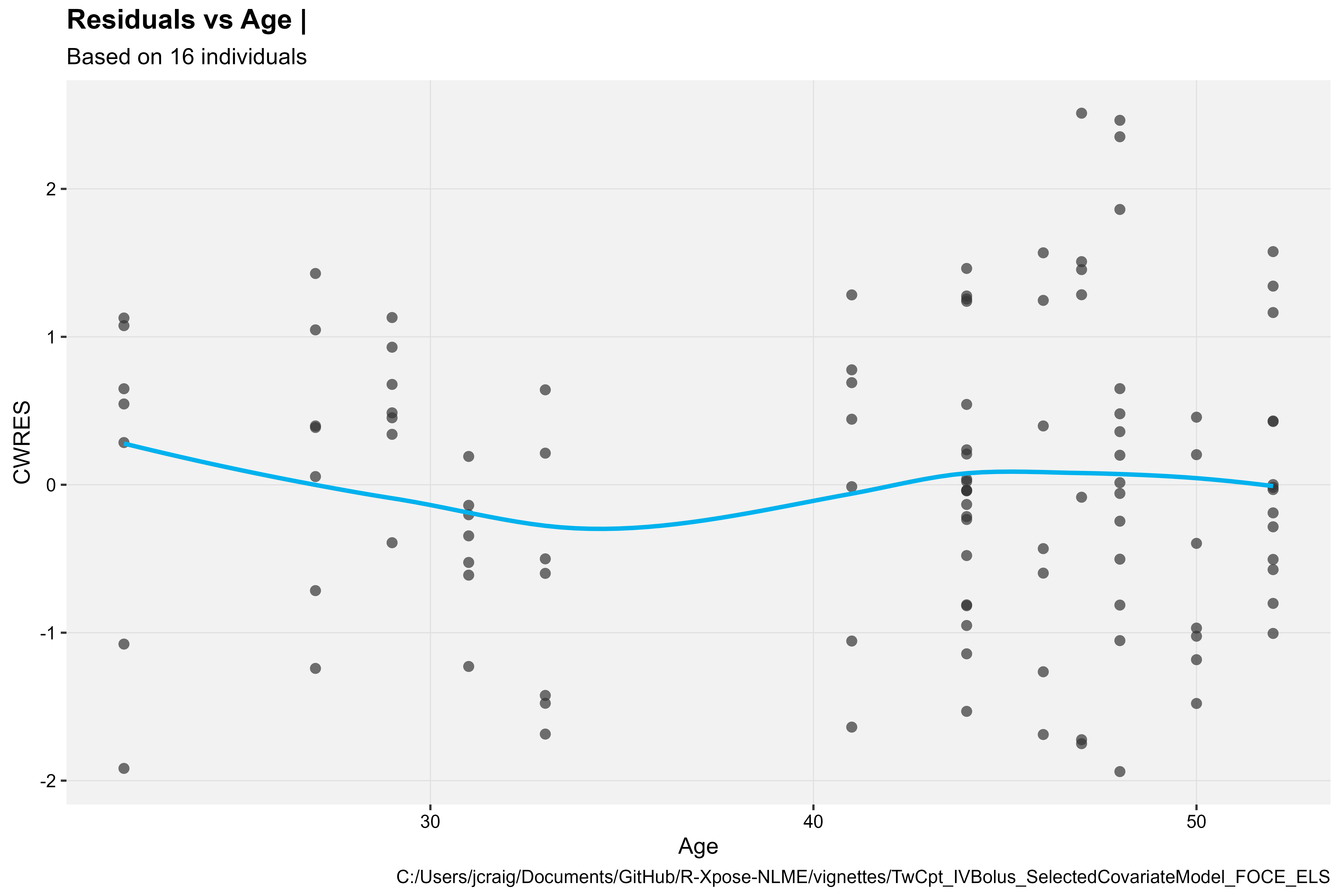
CWRES vs Categorical Covariate
library(Certara.Xpose.NLME)

res_vs_cov(xpdb, covariate = "Sex", res = "CWRES", type = "b")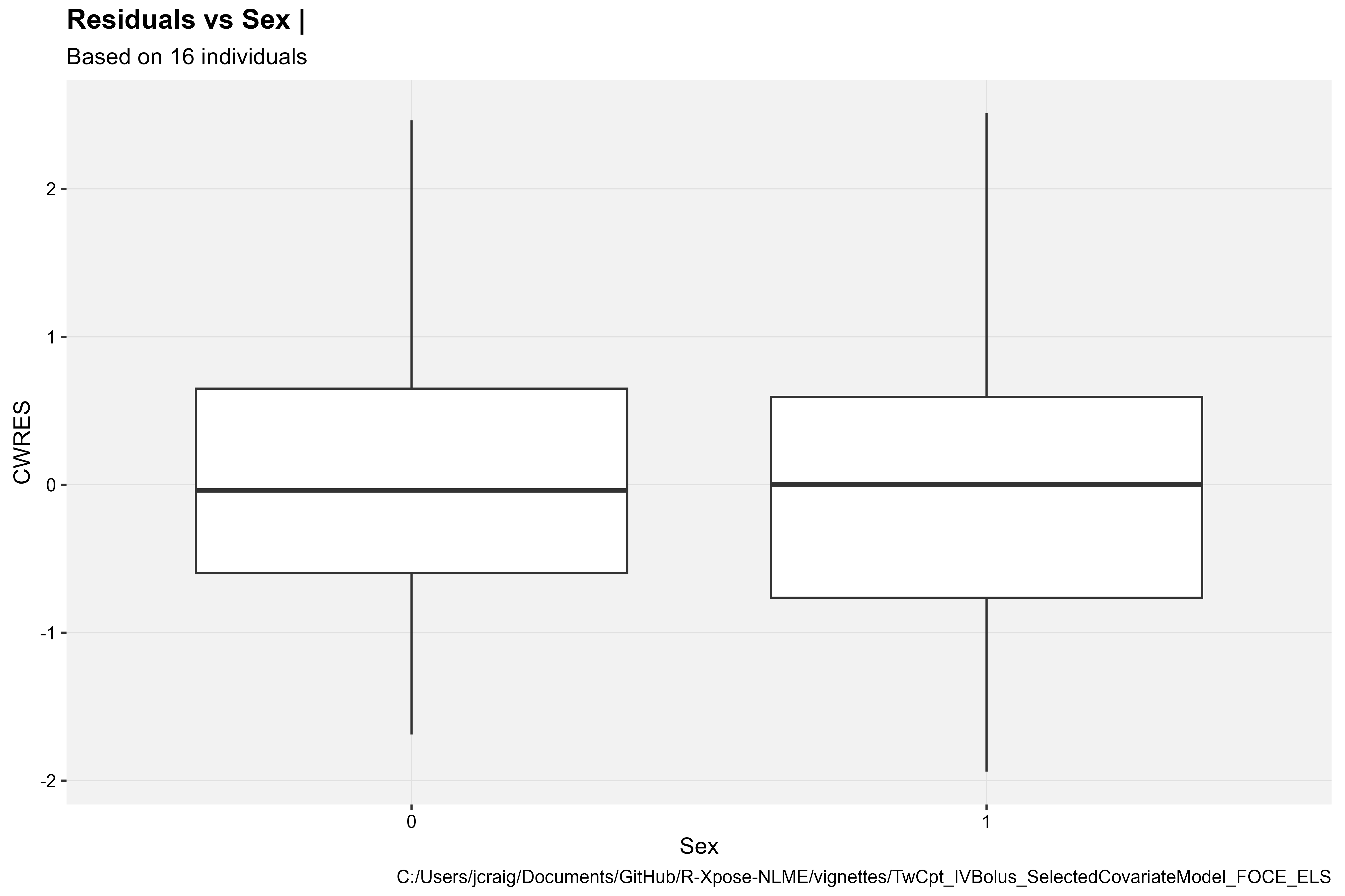
Extending with ggplot2
Add reference line
library(Certara.Xpose.NLME)
library(ggplot2)

res_vs_cov(xpdb, covariate = "BW", res = "CWRES", type = "ps") +
  geom_hline(yintercept = 0, linetype = "dashed", lwd = 1, color = "red") +
  theme_bw2()
#> `geom_smooth()` using formula = 'y ~ x'
#> `geom_smooth()` using formula = 'y ~ x'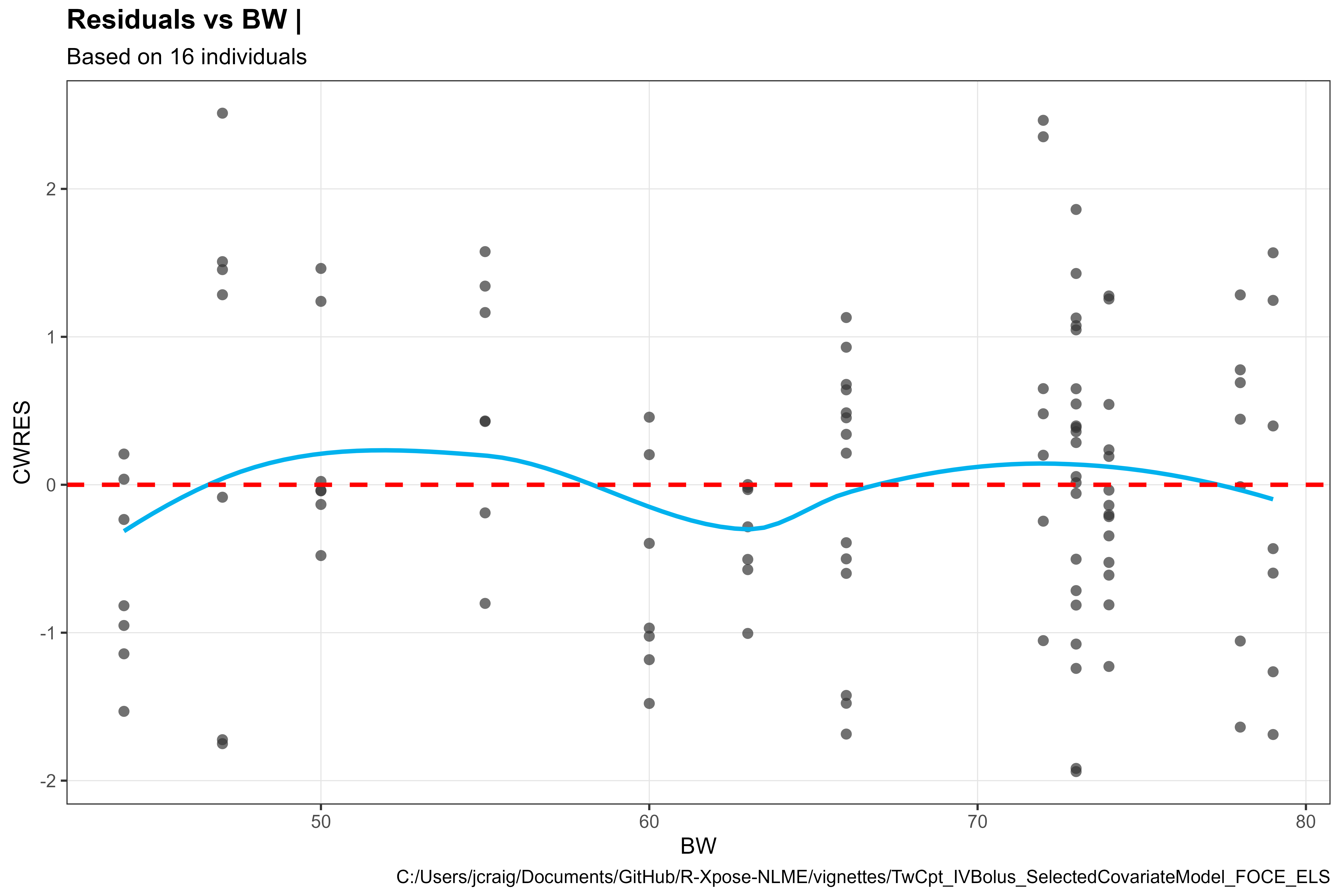
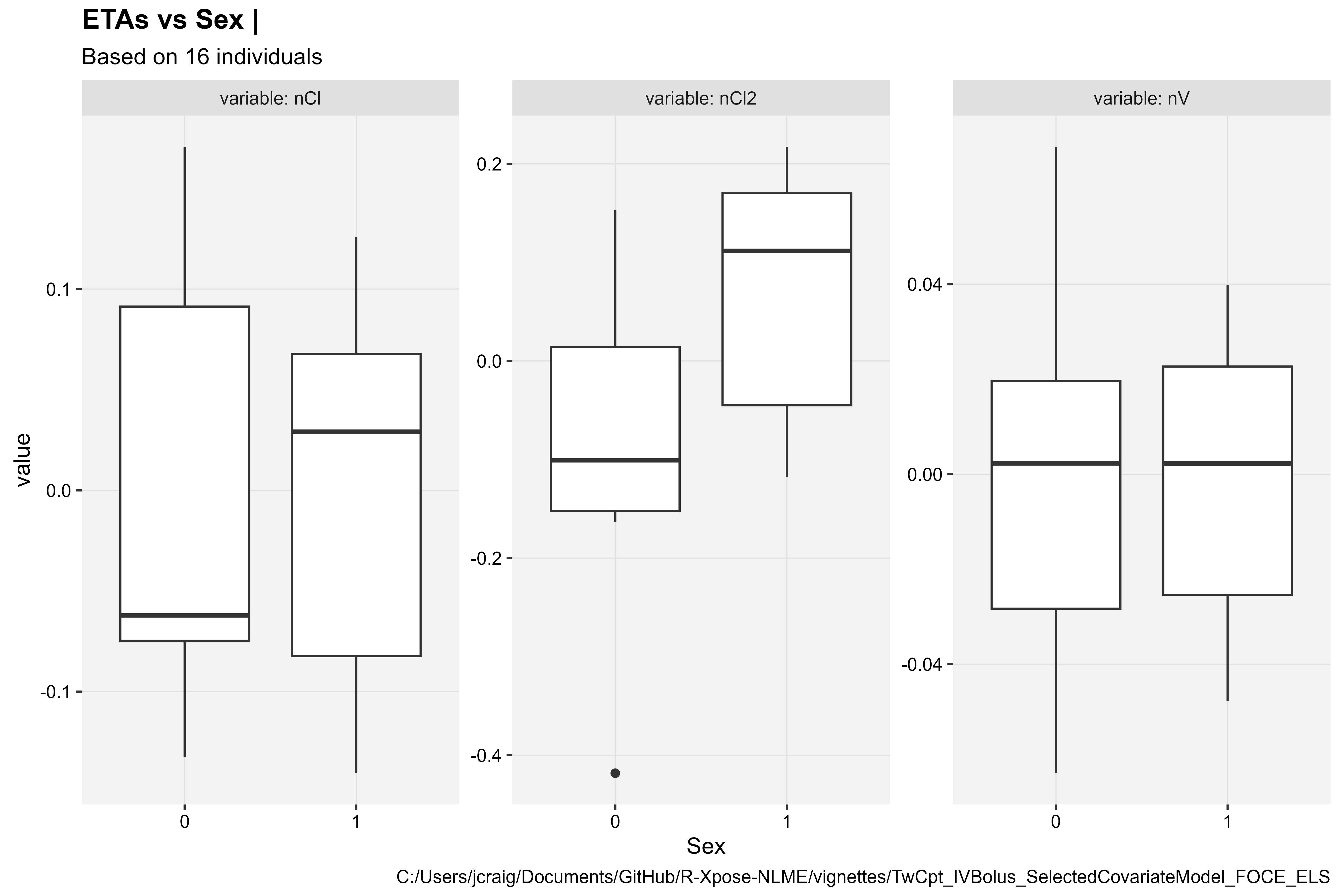
ETAs vs Covariates
ETAs vs Continuous Covariate
eta_vs_cov(xpdb, covariate = "Age", type = "ps")
#> `geom_smooth()` using formula = 'y ~ x'
#> `geom_smooth()` using formula = 'y ~ x'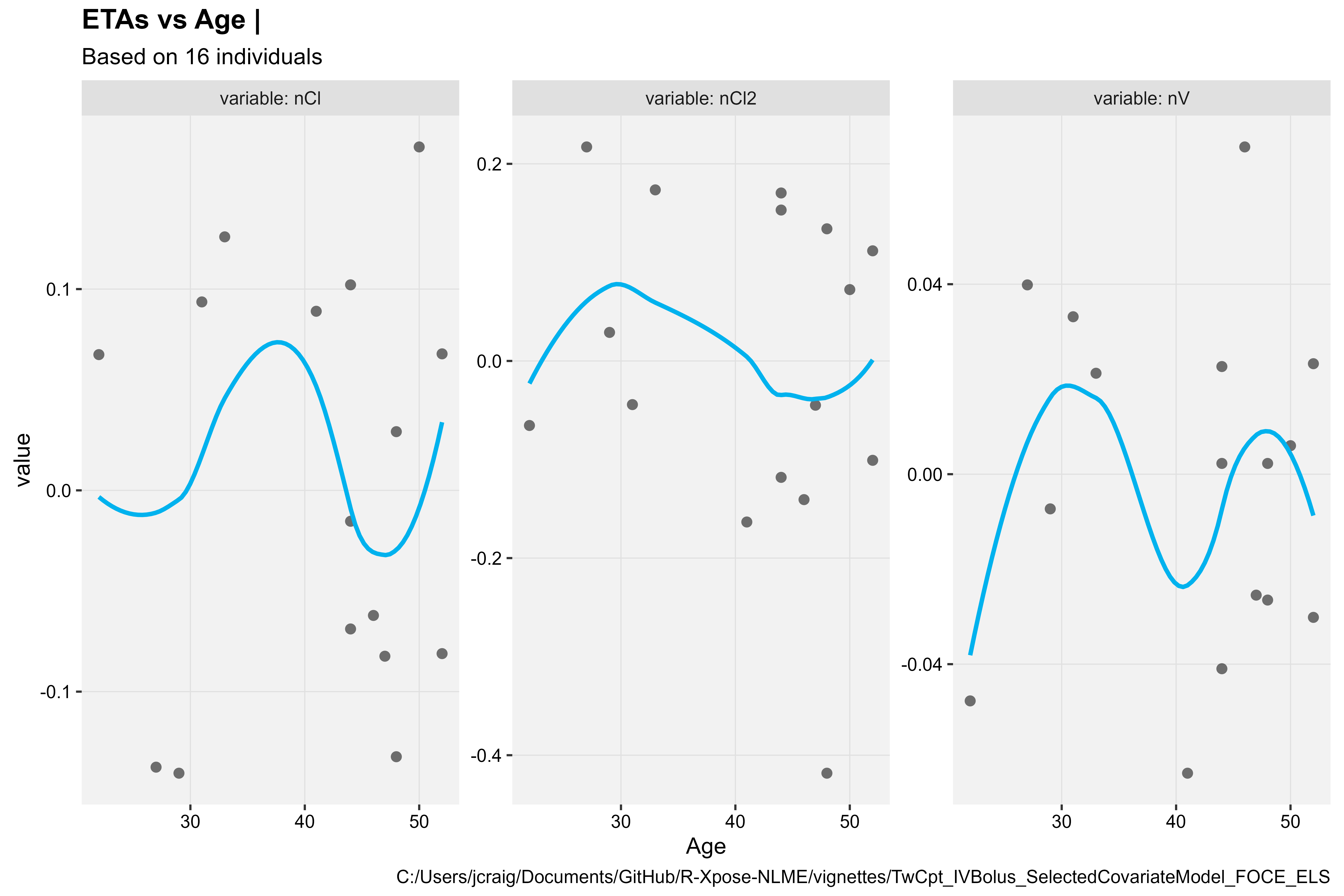
Structural Parameters vs Covariates
Structural Parameters vs Continuous Covariate
prm_vs_cov(xpdb, covariate = "BW", type = "ps")
#> `geom_smooth()` using formula = 'y ~ x'
#> `geom_smooth()` using formula = 'y ~ x'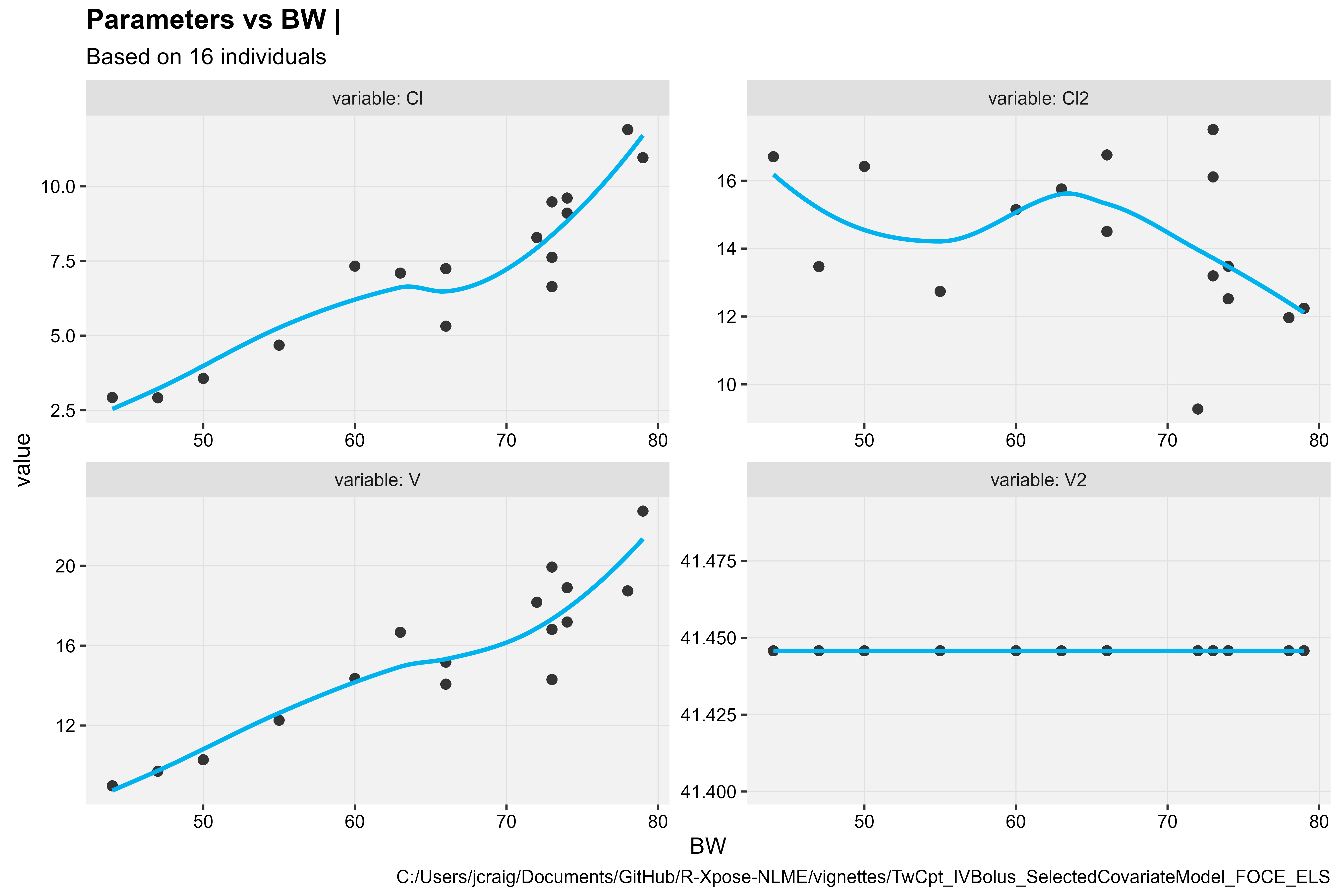
Structural Parameters vs Categorical Covariate
prm_vs_cov(xpdb, covariate = "Sex", type = "b")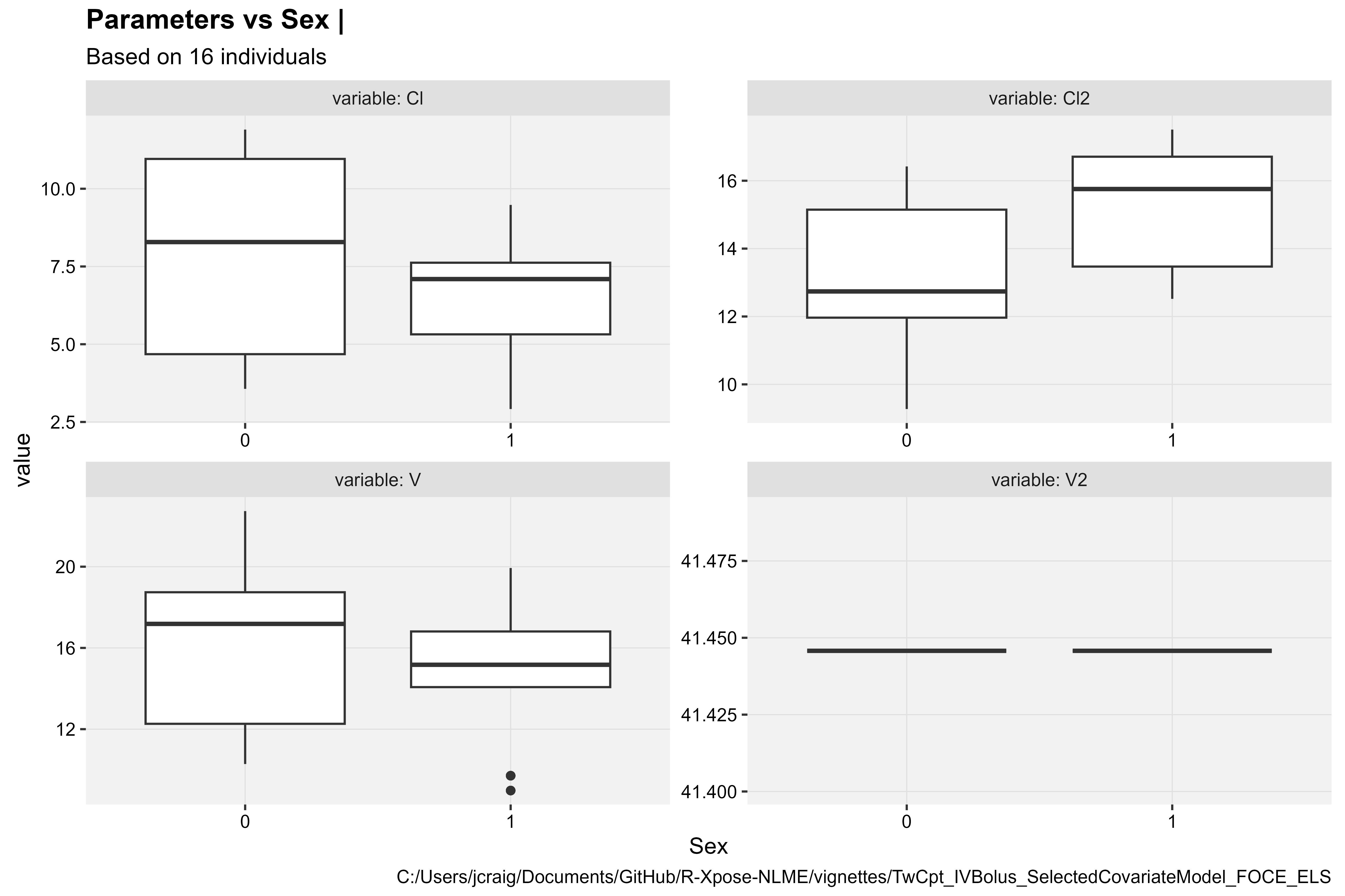
Note: We can remove the variable V2 from the
plots, which has a fixed value, by including the argument
drop_fixed = TRUE.
Using ggcertara
ggcertara is an R package to provide a standardized look
for plots employed by pharmacometricians. It provides a ggplot2 theme,
color palette, and a collection of plotting functions for basic
goodness-of-fit diagnostic plots.
Goodness-of-fit (GOF) data can easily be extracted from the
xpose_data object in order to utilize plot functions from
ggcertara.
For ggcertara installation and usage details, visit the
following link.
To learn more about the standardized set of basic goodness-of-fit
diagnostic plots available in ggcertara, explore the
following vignette.
library(ggcertara)
#> Registered S3 method overwritten by 'ggcertara':
#>   method from
#>   &.gg   patchwork

gofData <- xpose::get_data(xpdb)

colnames(gofData) <- tolower(colnames(gofData)) # ggcertara expects lower case column names

glimpse(gofData)
#> Rows: 112
#> Columns: 34
#> $ subject    <int> 1, 1, 1, 1, 1, 1, 1, 2, 2, 2, 2, 2, 2, 2, 3, 3, 3, 3, 3, 3,…
#> $ nom_time   <int> 0, 1, 1, 2, 4, 8, 24, 0, 1, 1, 2, 4, 8, 24, 0, 1, 1, 2, 4, …
#> $ act_time   <dbl> 0.00, 0.26, 1.10, 2.10, 4.13, 8.17, 23.78, 0.00, 0.37, 0.83…
#> $ amount     <int> 25000, NA, NA, NA, NA, NA, NA, 25000, NA, NA, NA, NA, NA, N…
#> $ conc       <dbl> 2010.0, 1330.0, 565.0, 216.0, 180.0, 120.0, 16.9, 850.0, 79…
#> $ bodyweight <int> 73, 73, 73, 73, 73, 73, 73, 79, 79, 79, 79, 79, 79, 79, 63,…
#> $ gender     <chr> "male", "male", "male", "male", "male", "male", "male", "fe…
#> $ id         <fct> 1, 1, 1, 1, 1, 1, 1, 2, 2, 2, 2, 2, 2, 2, 3, 3, 3, 3, 3, 3,…
#> $ whichreset <dbl> 0, 0, 0, 0, 0, 0, 0, 0, 0, 0, 0, 0, 0, 0, 0, 0, 0, 0, 0, 0,…
#> $ time       <dbl> 0.00, 0.26, 1.10, 2.10, 4.13, 8.17, 23.78, 0.00, 0.37, 0.83…
#> $ sex        <fct> 1, 1, 1, 1, 1, 1, 1, 0, 0, 0, 0, 0, 0, 0, 1, 1, 1, 1, 1, 1,…
#> $ age        <dbl> 22, 22, 22, 22, 22, 22, 22, 46, 46, 46, 46, 46, 46, 46, 52,…
#> $ bw         <dbl> 73, 73, 73, 73, 73, 73, 73, 79, 79, 79, 79, 79, 79, 79, 63,…
#> $ v          <dbl> 14.28920, 14.28920, 14.28920, 14.28920, 14.28920, 14.28920,…
#> $ cl         <dbl> 7.620701, 7.620701, 7.620701, 7.620701, 7.620701, 7.620701,…
#> $ v2         <dbl> 41.44075, 41.44075, 41.44075, 41.44075, 41.44075, 41.44075,…
#> $ cl2        <dbl> 13.19784, 13.19784, 13.19784, 13.19784, 13.19784, 13.19784,…
#> $ ivar       <dbl> 0.00, 0.26, 1.10, 2.10, 4.13, 8.17, 23.78, 0.00, 0.37, 0.83…
#> $ tad        <dbl> 0.00, 0.26, 1.10, 2.10, 4.13, 8.17, 23.78, 0.00, 0.37, 0.83…
#> $ pred       <dbl> 1669.82000, 1168.97000, 460.14600, 254.45900, 174.78100, 11…
#> $ ipred      <dbl> 1749.5700, 1211.1000, 455.1430, 239.9620, 160.2920, 105.393…
#> $ dv         <dbl> 2010.0, 1330.0, 565.0, 216.0, 180.0, 120.0, 16.9, 850.0, 79…
#> $ ires       <dbl> 260.42700, 118.90400, 109.85700, -23.96240, 19.70750, 14.60…
#> $ predse     <dbl> 0, 0, 0, 0, 0, 0, 0, 0, 0, 0, 0, 0, 0, 0, 0, 0, 0, 0, 0, 0,…
#> $ weight     <dbl> 3.26690e-07, 6.81778e-07, 4.82730e-06, 1.73665e-05, 3.89201…
#> $ iwres      <dbl> 0.937045, 0.618054, 1.519450, -0.628629, 0.773975, 0.872488…
#> $ wres       <dbl> 1.1638400, 0.6659370, 1.0869000, -1.0148200, 0.4876820, 0.2…
#> $ cwres      <dbl> 1.116910000, 0.645102000, 1.079270000, -1.074210000, 0.5454…
#> $ obsname    <fct> CObs, CObs, CObs, CObs, CObs, CObs, CObs, CObs, CObs, CObs,…
#> $ whichdose  <dbl> 1, 1, 1, 1, 1, 1, 1, 1, 1, 1, 1, 1, 1, 1, 1, 1, 1, 1, 1, 1,…
#> $ nv         <dbl> -0.04665681, -0.04665681, -0.04665681, -0.04665681, -0.0466…
#> $ ncl        <dbl> 0.06714209, 0.06714209, 0.06714209, 0.06714209, 0.06714209,…
#> $ ncl2       <dbl> -0.06544842, -0.06544842, -0.06544842, -0.06544842, -0.0654…
#> $ evid       <dbl> 0, 0, 0, 0, 0, 0, 0, 0, 0, 0, 0, 0, 0, 0, 0, 0, 0, 0, 0, 0,…
Basic GOF
Use the gof() function to plot basic GOF plot with
default panel options.
gof(gofData)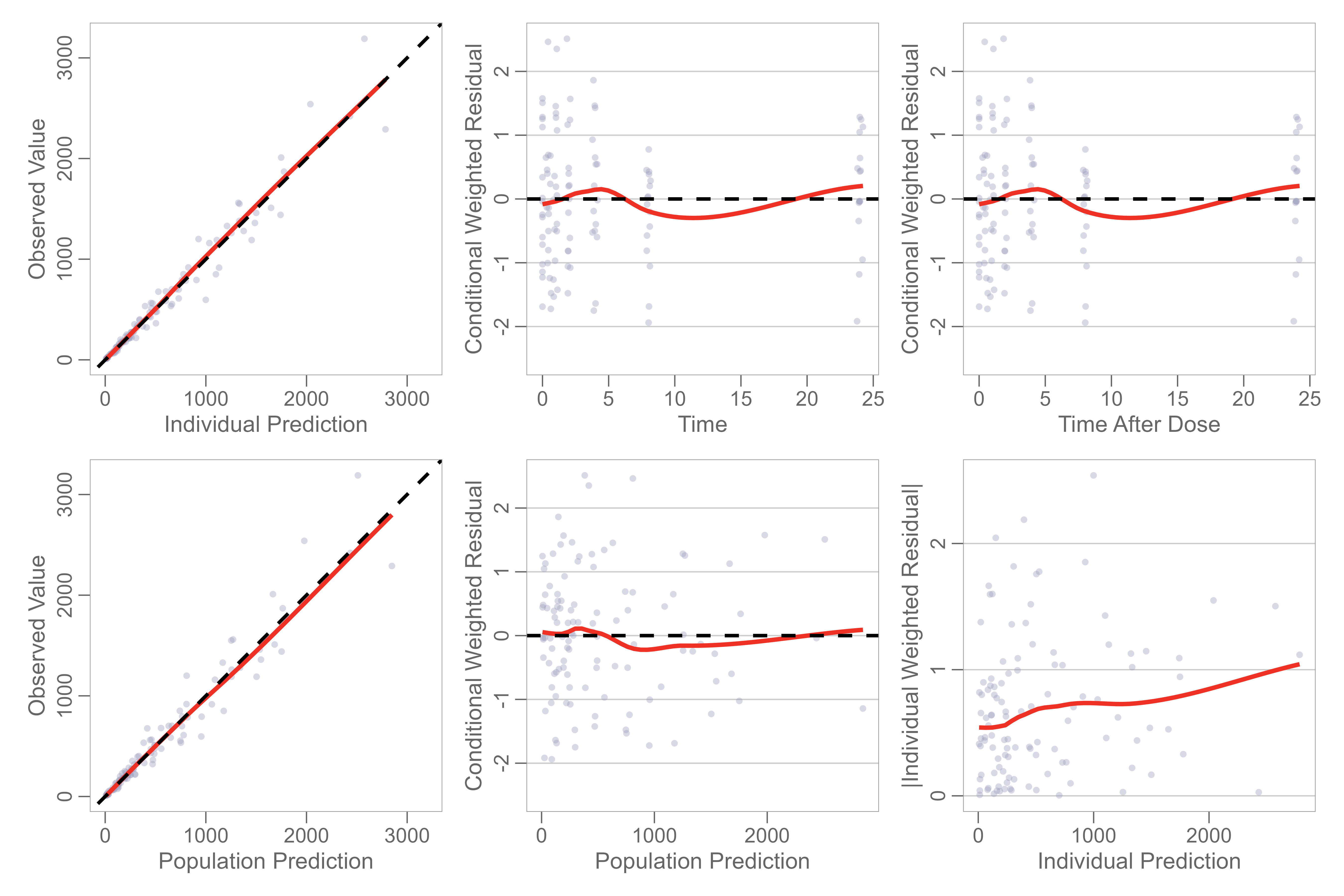
You may select from different combinations of gof plots using the
panels argument.
gof(gofData, panels = 3:6)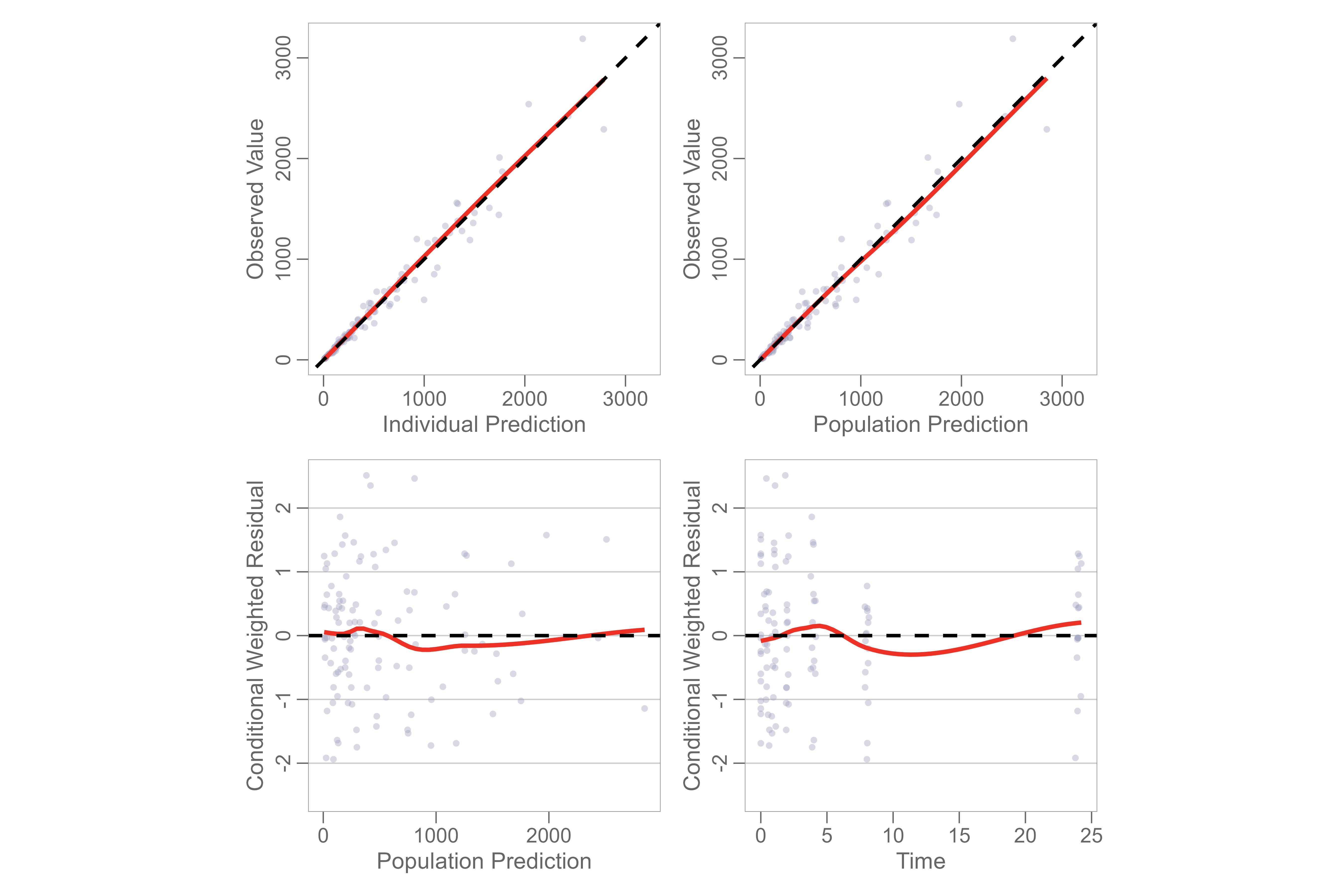
Color Explorer
The ggcertara package contains a useful Shiny
application to explore different color palettes and test how those with
color blindness will perceive your selected colors.
First, create the plot and assign a return value.
myplot <- gof(gofData)Next, pass the plot to the plotobj argument in
run_colorexplorer().
run_colorexplorer(plotobj = myplot)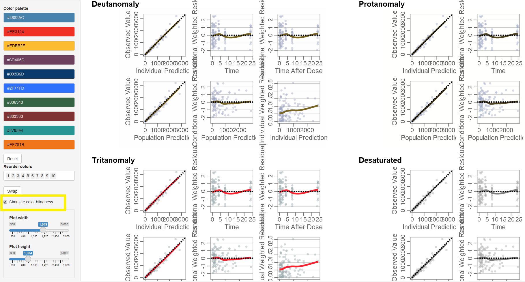
To simulate color blindness given the colors chosen in the palette, click the checkbox labeled “Simulate Color Blindness”.