Exploring Covariate Search Results
scm_access.RmdBoth shotgunSearch() and stepwiseSearch()
archive per-scenario results automatically. After a search completes you
can recover the fitted model and diagnostics for any scenario without
re-running the search. This vignette walks through the archive-access
workflow:
- Inspect the search result and its custom
print()output - Use
scmSearchTable()for a presentation data frame (table formatters) - Use
listSCMRuns()to discover archived scenarios - Use
getSCMResults()to retrieve a model and fit output - Pass the retrieved results to
Certara.Xpose.NLMEfor diagnostics
library(Certara.RsNLME)
library(magrittr) # `%>%`
The chunks below execute live NLME searches and require the NLME engine (
INSTALLDIRenv var pointing at a valid install). When that is not available — e.g. CRAN / CI vignette builds — the chunks are skipped.
Setup
Create a writable working directory and configure a local multicore host. All model files, search outputs, and archives will be written here.
workingDir <- file.path(tempdir(), "scm_access_vignette")
dir.create(workingDir, recursive = TRUE, showWarnings = FALSE)

host <- hostParams(
  sharedDirectory = workingDir,
  parallelMethod = "Multicore",
  numCores = 4
)
Build a base model with covariates
We use the built-in pkData dataset (16 subjects, single
bolus dose) and a two-compartment model. BodyWeight
(continuous) and Gender (categorical) are added as
candidate covariates on V and Cl.
baseModel <- pkmodel(
  numCompartments = 2,
  data = pkData,
  ID = "Subject",
  Time = "Act_Time",
  A1 = "Amount",
  CObs = "Conc",
  workingDir = workingDir
)

baseModel <- baseModel %>%
  addCovariate(
    covariate = "BodyWeight",
    type = "Continuous",
    effect = c("V", "Cl"),
    direction = "Forward",
    center = "Mean"
  ) %>%
  addCovariate(
    covariate = "Gender",
    type = "Categorical",
    effect = c("V", "Cl"),
    levels = c(0, 1),
    labels = c("male", "female")
  )
covariateModel(baseModel)
#> An object of class "CovariateEffectModel"
#> Slot "numCovariates":
#> [1] 4
#>
#> Slot "covariateList":
#> [1] "V-BodyWeight,V-Gender,Cl-BodyWeight,Cl-Gender"
#>
#> Slot "scenarioNames":
#> [1] "S,S,S,S"
#>
#> Slot "isDefault":
#> [1] "1,1,1,1"
#>
#> Slot "degreesOfFreedom":
#> [1] "1,1,1,1"
#>
#> Slot "enableIDs":
#> [1] "0,1,2,3"
Run a shotgun search
Shotgun search evaluates every combination of enabled covariate effects in parallel. We use Naive-Pooled estimation here for speed.
shotgunModel <- copyModel(baseModel, modelName = "shotgunModel")

params <- engineParams(baseModel, method = "Naive-Pooled")

shotgunResult <- shotgunSearch(
  model = shotgunModel,
  hostPlatform = host,
  covariateModel = covariateModel(shotgunModel),
  params = params
)
The return value is a data frame with an scmSearchResult
S3 class. Printing it shows a header, the best scenario’s criteria, and
a ranked table of scenarios. Fit criteria (-2LL,
AIC, BIC) and the best flag are
columns of this data frame. Use getSCMResults() to retrieve
the fitted model for any row:
print(shotgunResult)
#> Shotgun Covariate Search Results
#> -------------------------------------------
#> Run folder : /myproject/shotgunModel/shotgun_20260902_112324
#> Scenarios  : 16 evaluated, 1 best
#>
#> Best Scenario (by -2LL)
#> -------------------------------------------
#> Scenario  : cshot015 V-BodyWeight V-Gender Cl-BodyWeight Cl-Gender
#> -2LL      : 1245.95
#> AIC       : 1263.95
#> BIC       : 1288.42
#>
#> Scenario Ranking by -2LL (top 10 of 16)
#> -------------------------------------------
#>    Scenario                                                  -2LL     AIC     BIC
#>  * cshot015 V-BodyWeight V-Gender Cl-BodyWeight Cl-Gender 1245.95 1263.95 1288.42
#>    cshot013 V-BodyWeight Cl-BodyWeight Cl-Gender           1246.3  1262.3 1284.05
#>    cshot007 V-BodyWeight V-Gender Cl-BodyWeight           1260.83 1276.83 1298.57
#>    cshot005 V-BodyWeight Cl-BodyWeight                    1261.04 1275.04 1294.07
#>    cshot014 V-Gender Cl-BodyWeight Cl-Gender              1268.98 1284.98 1306.73
#>    cshot012 Cl-BodyWeight Cl-Gender                       1269.75 1283.75 1302.78
#>    cshot006 V-Gender Cl-BodyWeight                        1281.56 1295.56 1314.59
#>    cshot004 Cl-BodyWeight                                 1281.57 1293.57 1309.88
#>    cshot011 V-BodyWeight V-Gender Cl-Gender               1396.49 1412.49 1434.24
#>    cshot009 V-BodyWeight Cl-Gender                        1396.62 1410.62 1429.65
#> (... 6 more scenarios)
#>
#> Use getSCMResults() to retrieve the final model for a scenario.
#>
#> Engine: Naive-Pooled | Runtime: 50.32 s | RsNLME: 3.2.0
The searchRunDir attribute connects the result to its
archive folder on disk. Downstream functions like
listSCMRuns() and getSCMResults() use it to
locate the archive:
attr(shotgunResult, "searchRunDir")
#> [1] "/myproject/shotgunModel/shotgun_20260407_143022"
Run a stepwise search
Stepwise search adds and removes effects sequentially based on
statistical thresholds. When stepwiseParams is omitted, the
defaults are used (add threshold 0.01, remove threshold 0.001, method
-2LL).
stepwiseModel <- copyModel(baseModel, modelName = "stepwiseModel")

stepwiseResult <- stepwiseSearch(
  model = stepwiseModel,
  hostPlatform = host,
  covariateModel = covariateModel(stepwiseModel),
  params = params
)
The stepwise print uses the same ranking layout as shotgun. The
* marker is the scenario selected by the stepwise search,
which need not be the global minimum of -2LL:
print(stepwiseResult)
#> Stepwise Covariate Search Results
#> -------------------------------------------
#> Run folder : /myproject/stepwiseModel/stepwise_20260902_112415
#> Scenarios  : 12 evaluated, 1 best
#>
#> Best Scenario (selected by stepwise search)
#> -------------------------------------------
#> Scenario  : cstep009  V-BodyWeight Cl-BodyWeight Cl-Gender
#> -2LL      : 1246.3
#> AIC       : 1262.3
#> BIC       : 1284.05
#>
#> Scenario Ranking by -2LL (top 10 of 12)
#> -------------------------------------------
#>    Scenario                                                   -2LL     AIC     BIC
#>    cstep010  V-BodyWeight V-Gender Cl-BodyWeight Cl-Gender 1245.95 1263.95 1288.42
#>  * cstep009  V-BodyWeight Cl-BodyWeight Cl-Gender           1246.3  1262.3 1284.05
#>    cstep008  V-BodyWeight V-Gender Cl-BodyWeight           1260.83 1276.83 1298.57
#>    cstep005  V-BodyWeight Cl-BodyWeight                    1261.04 1275.04 1294.07
#>    cstep007  Cl-BodyWeight Cl-Gender                       1269.75 1283.75 1302.78
#>    cstep006  V-Gender Cl-BodyWeight                        1281.56 1295.56 1314.59
#>    cstep003  Cl-BodyWeight                                 1281.57 1293.57 1309.88
#>    cstep011  V-BodyWeight Cl-Gender                        1396.62 1410.62 1429.65
#>    cstep001  V-BodyWeight                                   1399.8  1411.8 1428.11
#>    cstep004  Cl-Gender                                     1401.34 1413.34 1429.66
#> (... 2 more scenarios)
#>
#> Use getSCMResults() to retrieve the final model for a scenario.
#>
#> Engine: Naive-Pooled | Runtime: 59.60 s | RsNLME: 3.2.0
Presentation tables
print() stays compact. For a decision table (stepwise)
or a ranking table that includes the enabled covariate effects
(shotgun), use scmSearchTable().
Certara.RsNLME does not import flextable; the
chunks below render with it when that package is installed.
tab <- scmSearchTable(stepwiseResult)Step |
Direction |
Scenario |
Model |
CovEffects |
Base -2LL |
New -2LL |
d-2LL |
Goal |
Chosen |
PVal |
|---|---|---|---|---|---|---|---|---|---|---|
1 |
Forward - Addition |
cstep001 V-BodyWeight |
dVdBodyWeight |
dVdBodyWeight |
1,404.430 |
1,399.799 |
4.63106 |
6.634897 |
N |
0.0313981595477371006053246560441039036959 |
1 |
Forward - Addition |
cstep002 V-Gender |
dVdGender1 |
dVdGender1 |
1,404.430 |
1,404.336 |
0.09368 |
6.634897 |
N |
0.7595499123390919704590373839891981333494 |
1 |
Forward - Addition |
cstep003 Cl-BodyWeight |
dCldBodyWeight |
dCldBodyWeight |
1,404.430 |
1,281.572 |
122.85806 |
6.634897 |
Y |
0.0000000000000000000000000001497903197577 |
1 |
Forward - Addition |
cstep004 Cl-Gender |
dCldGender1 |
dCldGender1 |
1,404.430 |
1,401.345 |
3.08530 |
6.634897 |
N |
0.0790026950672650940532548702321946620941 |
2 |
Forward - Addition |
cstep005 V-BodyWeight Cl-BodyWeight |
dVdBodyWeight |
dVdBodyWeight,dCldBodyWeight |
1,281.572 |
1,261.041 |
20.53108 |
6.634897 |
Y |
0.0000058670830659168902877081963609384729 |
2 |
Forward - Addition |
cstep006 V-Gender Cl-BodyWeight |
dVdGender1 |
dVdGender1,dCldBodyWeight |
1,281.572 |
1,281.557 |
0.01456 |
6.634897 |
N |
0.9039565209256029687523437132767867296934 |
2 |
Forward - Addition |
cstep007 Cl-BodyWeight Cl-Gender |
dCldGender1 |
dCldBodyWeight,dCldGender1 |
1,281.572 |
1,269.755 |
11.81742 |
6.634897 |
N |
0.0005867911400608549765678390031098388135 |
3 |
Forward - Addition |
cstep008 V-BodyWeight V-Gender Cl-BodyWeight |
dVdGender1 |
dVdBodyWeight,dVdGender1,dCldBodyWeight |
1,261.041 |
1,260.827 |
0.21394 |
6.634897 |
N |
0.6436966444703150491690735179872717708349 |
3 |
Forward - Addition |
cstep009 V-BodyWeight Cl-BodyWeight Cl-Gender |
dCldGender1 |
dVdBodyWeight,dCldBodyWeight,dCldGender1 |
1,261.041 |
1,246.298 |
14.74252 |
6.634897 |
Y |
0.0001232354605057110058519143080957292113 |
4 |
Forward - Addition |
cstep010 V-BodyWeight V-Gender Cl-BodyWeight Cl-Gender |
dVdBodyWeight,dVdGender1,dCldBodyWeight,dCldGender1 |
dVdBodyWeight,dVdGender1,dCldBodyWeight,dCldGender1 |
1,246.298 |
1,245.949 |
0.34948 |
6.634897 |
N |
0.5544076371351650545094003064150456339121 |
5 |
Backward - Deletion |
cstep007 Cl-BodyWeight Cl-Gender |
dVdBodyWeight |
dCldBodyWeight,dCldGender1 |
1,246.298 |
1,269.755 |
-23.45618 |
10.827566 |
N |
0.0000012779155024537500306286430529212339 |
5 |
Backward - Deletion |
cstep011 V-BodyWeight Cl-Gender |
dCldBodyWeight |
dVdBodyWeight,dCldGender1 |
1,246.298 |
1,396.622 |
-150.32324 |
10.827566 |
N |
0.0000000000000000000000000000000001473356 |
5 |
Backward - Deletion |
cstep005 V-BodyWeight Cl-BodyWeight |
dCldGender1 |
dVdBodyWeight,dCldBodyWeight |
1,246.298 |
1,261.041 |
-14.74252 |
10.827566 |
N |
0.0001232354605057110058519143080957292113 |
Shotgun results produce a ranking table with a
CovEffects column joined from the archive:
shotgunTab <- scmSearchTable(shotgunResult)Scenario |
CovEffects |
-2LL |
AIC |
BIC |
best |
|---|---|---|---|---|---|
cshot000 |
1,404.430 |
1,414.430 |
1,428.022 |
N |
|
cshot001 V-BodyWeight |
dVdBodyWeight |
1,399.799 |
1,411.799 |
1,428.110 |
N |
cshot002 V-Gender |
dVdGender1 |
1,404.336 |
1,416.336 |
1,432.647 |
N |
cshot003 V-BodyWeight V-Gender |
dVdBodyWeight,dVdGender1 |
1,399.753 |
1,413.753 |
1,432.782 |
N |
cshot004 Cl-BodyWeight |
dCldBodyWeight |
1,281.572 |
1,293.572 |
1,309.883 |
N |
cshot005 V-BodyWeight Cl-BodyWeight |
dVdBodyWeight,dCldBodyWeight |
1,261.041 |
1,275.041 |
1,294.070 |
N |
cshot006 V-Gender Cl-BodyWeight |
dVdGender1,dCldBodyWeight |
1,281.557 |
1,295.557 |
1,314.587 |
N |
cshot007 V-BodyWeight V-Gender Cl-BodyWeight |
dVdBodyWeight,dVdGender1,dCldBodyWeight |
1,260.827 |
1,276.827 |
1,298.575 |
N |
cshot008 Cl-Gender |
dCldGender1 |
1,401.345 |
1,413.345 |
1,429.656 |
N |
cshot009 V-BodyWeight Cl-Gender |
dVdBodyWeight,dCldGender1 |
1,396.622 |
1,410.622 |
1,429.651 |
N |
cshot010 V-Gender Cl-Gender |
dVdGender1,dCldGender1 |
1,401.063 |
1,415.063 |
1,434.093 |
N |
cshot011 V-BodyWeight V-Gender Cl-Gender |
dVdBodyWeight,dVdGender1,dCldGender1 |
1,396.493 |
1,412.493 |
1,434.241 |
N |
cshot012 Cl-BodyWeight Cl-Gender |
dCldBodyWeight,dCldGender1 |
1,269.755 |
1,283.755 |
1,302.784 |
N |
cshot013 V-BodyWeight Cl-BodyWeight Cl-Gender |
dVdBodyWeight,dCldBodyWeight,dCldGender1 |
1,246.298 |
1,262.298 |
1,284.046 |
N |
cshot014 V-Gender Cl-BodyWeight Cl-Gender |
dVdGender1,dCldBodyWeight,dCldGender1 |
1,268.977 |
1,284.977 |
1,306.725 |
N |
cshot015 V-BodyWeight V-Gender Cl-BodyWeight Cl-Gender |
dVdBodyWeight,dVdGender1,dCldBodyWeight,dCldGender1 |
1,245.949 |
1,263.949 |
1,288.415 |
Y |
Browse archived scenarios
listSCMRuns() discovers archived SCM folders and returns
a data frame with one row per scenario. It accepts several types of
input.
From a search result
Pass the result data frame directly — listSCMRuns() uses
its searchRunDir attribute:
shotgunRuns <- listSCMRuns(shotgunResult)
shotgunRuns[, c("Scenario", "enableFlags", "status")]
#>                                                  Scenario enableFlags  status
#> 1                                                cshot000             SUCCESS
#> 2                                   cshot001 V-BodyWeight           0 SUCCESS
#> 3                                       cshot002 V-Gender           1 SUCCESS
#> 4                          cshot003 V-BodyWeight V-Gender         0,1 SUCCESS
#> 5                                  cshot004 Cl-BodyWeight           2 SUCCESS
#> 6                     cshot005 V-BodyWeight Cl-BodyWeight         0,2 SUCCESS
#> 7                         cshot006 V-Gender Cl-BodyWeight         1,2 SUCCESS
#> 8            cshot007 V-BodyWeight V-Gender Cl-BodyWeight       0,1,2 SUCCESS
#> 9                                      cshot008 Cl-Gender           3 SUCCESS
#> 10                        cshot009 V-BodyWeight Cl-Gender         0,3 SUCCESS
#> 11                            cshot010 V-Gender Cl-Gender         1,3 SUCCESS
#> 12               cshot011 V-BodyWeight V-Gender Cl-Gender       0,1,3 SUCCESS
#> 13                       cshot012 Cl-BodyWeight Cl-Gender         2,3 SUCCESS
#> 14          cshot013 V-BodyWeight Cl-BodyWeight Cl-Gender       0,2,3 SUCCESS
#> 15              cshot014 V-Gender Cl-BodyWeight Cl-Gender       1,2,3 SUCCESS
#> 16 cshot015 V-BodyWeight V-Gender Cl-BodyWeight Cl-Gender     0,1,2,3 SUCCESS
From a model object
Pass an NlmePmlModel — listSCMRuns() scans
the model’s working directory for SCM archive folders:
listSCMRuns(shotgunModel)[, c("Scenario", "enableFlags", "status")]
#>                                                  Scenario enableFlags  status
#> 1                                                cshot000             SUCCESS
#> 2                                   cshot001 V-BodyWeight           0 SUCCESS
#> 3                                       cshot002 V-Gender           1 SUCCESS
#> 4                          cshot003 V-BodyWeight V-Gender         0,1 SUCCESS
#> 5                                  cshot004 Cl-BodyWeight           2 SUCCESS
#> 6                     cshot005 V-BodyWeight Cl-BodyWeight         0,2 SUCCESS
#> 7                         cshot006 V-Gender Cl-BodyWeight         1,2 SUCCESS
#> 8            cshot007 V-BodyWeight V-Gender Cl-BodyWeight       0,1,2 SUCCESS
#> 9                                      cshot008 Cl-Gender           3 SUCCESS
#> 10                        cshot009 V-BodyWeight Cl-Gender         0,3 SUCCESS
#> 11                            cshot010 V-Gender Cl-Gender         1,3 SUCCESS
#> 12               cshot011 V-BodyWeight V-Gender Cl-Gender       0,1,3 SUCCESS
#> 13                       cshot012 Cl-BodyWeight Cl-Gender         2,3 SUCCESS
#> 14          cshot013 V-BodyWeight Cl-BodyWeight Cl-Gender       0,2,3 SUCCESS
#> 15              cshot014 V-Gender Cl-BodyWeight Cl-Gender       1,2,3 SUCCESS
#> 16 cshot015 V-BodyWeight V-Gender Cl-BodyWeight Cl-Gender     0,1,2,3 SUCCESS
From a working directory path
You can also pass the model’s working directory path directly.
listSCMRuns() looks for shotgun_* /
stepwise_* subfolders at the top level of the given
path:
modelDir <- shotgunModel@modelInfo@workingDir
allRuns <- listSCMRuns(modelDir)
nrow(allRuns)
#> [1] 16
listSCMRuns() is a catalog of archived scenarios:
labels, enable flags, and status. Criteria and the
best flag stay on the search-result data frame
(shotgunResult / stepwiseResult). If any
scenario did not succeed, listSCMRuns() emits a message and
getSCMResults() of that row prints a Diagnostics block with
the engine error files.
See ?listSCMRuns for full column documentation.
Retrieve a specific scenario
getSCMResults() loads the archived base model,
reconstructs the scenario-specific model, and assembles a
fitmodel()-compatible output list. It returns three
elements:
-
model— the reconstructedNlmePmlModelwith accepted parameter estimates (or initial values when the fit did not converge) -
fitmodelOutput— a list compatible withfitmodel()output (residuals, convergence data,dmp.txt, etc.) -
scenarioInfo— a single-row data frame with scenario metadata
Best scenario (default)
When no selector is given, the best scenario is returned:
res <- getSCMResults(shotgunResult)Printing the result shows a compact fit summary, then the
reconstructed model PML (accepted parameter values from
final.mdl). If the scenario did not succeed, the Fit Output
block is replaced by Diagnostics (err2.txt,
nlme7engine.log, and related engine files) and the model
heading notes that the fit did not converge (PML comes from
wiped.mdl when final.mdl was never
written):
print(res)
#> Shotgun Scenario Result
#> -------------------------------------------
#> Scenario  : cshot015 V-BodyWeight V-Gender Cl-BodyWeight Cl-Gender
#> Status    : SUCCESS
#> -2LL      : 1245.95    AIC       : 1263.95    BIC       : 1288.42
#>
#> Fit Output
#> -------------------------------------------
#> Return code  : 1 (Convergence achieved)
#> nSubj/nObs   : 16 / 112
#> -2LL         : 1245.95
#>
#> Final Model (with accepted estimates)
#> -------------------------------------------
#>
#>  Model Overview
#>  -------------------------------------------
#> Model Name        :  shotgunModel
#> Working Directory :  C:/Users/jcraig/AppData/Local/Temp/RtmpEp6VEg/shotgunModel/shotgun_20260902_112324/cshot015__f
#> Is population     :  TRUE
#> Model Type        :  PK
#>
#>  PK
#>  -------------------------------------------
#> Parameterization  :  Clearance
#> Absorption        :  Intravenous
#> Num Compartments  :  2
#> Dose Tlag?        :  FALSE
#> Elimination Comp ?:  FALSE
#> Infusion Allowed ?:  FALSE
#> Sequential        :  FALSE
#> Freeze PK         :  FALSE
#>
#>  PML
#>  -------------------------------------------
#> test(){
#>     cfMicro(A1,Cl/V, Cl2/V, Cl2/V2)
#>     dosepoint(A1)
#>     C = A1 / V
#>     error(CEps=0.222467126691649)
#>     observe(CObs=C * ( 1 + CEps))
#>     stparm(V = tvV * ((BodyWeight/mean(BodyWeight))^dVdBodyWeight)   * exp(dVdGender1*(Gender==1)) * exp(nV))
#>     stparm(Cl = tvCl * ((BodyWeight/mean(BodyWeight))^dCldBodyWeight)   * exp(dCldGender1*(Gender==1)) * exp(nCl))
#>     stparm(V2 = tvV2 * exp(nV2))
#>     stparm(Cl2 = tvCl2 * exp(nCl2))
#>     fcovariate(BodyWeight)
#>     fcovariate(Gender())
#>     fixef(tvV = c(,15.0469923907693,))
#>     fixef(tvCl = c(,6.12329659194035,))
#>     fixef(tvV2 = c(,43.477839360019,))
#>     fixef(tvCl2 = c(,14.1825161412046,))
#>     fixef(dVdBodyWeight = c(,1.25376679263709,))
#>     fixef(dVdGender1 = c(,0.0551594624972583,))
#>     fixef(dCldBodyWeight = c(,2.26185396741583,))
#>     fixef(dCldGender1 = c(,0.173857038809218,))
#>     ranef(diag(nV,nCl,nV2,nCl2) = c(1,1,1,1))
#>
#> }
#>
#>  Structural Parameters
#>  -------------------------------------------
#>  V Cl V2 Cl2
#>  -------------------------------------------
#> Observations:
#> Observation Name :  CObs
#> Effect Name      :  C
#> Epsilon Name     :  CEps
#> Epsilon Type     :  Multiplicative
#> Epsilon frozen   :  FALSE
#> is BQL           :  FALSE
#>  -------------------------------------------
#>  Column Mappings
#>  -------------------------------------------
#> Model Variable Name : Data Column name
#> id                  : Subject
#> time                : Act_Time
#> A1                  : Amount
#> BodyWeight          : BodyWeight
#> Gender              : Gender( male=0 female=1 )
#> CObs                : Conc
#>
#>
#> Engine: Naive-Pooled | RsNLME: 3.2.0
For a programmatic digest of scenario metadata, criteria, and the
embedded fitmodelOutput header (engine, return code,
runtime, RsNLMEVersion) without the model PML, use
summary():
summary(res)The structured list returned by summary() is intended
for scripted downstream use; the print() method on the
summary renders the same fields as a compact console block. The
analogous summary(shotgunResult) /
summary(stepwiseResult) works on the search-result data
frame and surfaces the best scenario, top-N ranking, and the same
run-context fields.
Select by row
Pick any scenario from the listSCMRuns() output:
targetRow <- shotgunRuns[2, ]
res2 <- getSCMResults(targetRow)
res2$scenarioInfo$scenarioLabel
#> [1] "cshot001 V-BodyWeight"
Select by scenario label or enable IDs
When x resolves to an SCM folder (via a search result,
model, or folder path), you can also select by label or enable IDs:
getSCMResults(shotgunResult, scenario = "cshot006 V-Gender Cl-BodyWeight")

getSCMResults(shotgunResult, enableIDs = "1,3")
Model vs fitmodelOutput
The model and fitmodelOutput elements
represent two complementary views of the scenario:
modelcontains PML fromfinal.mdl— the wiped structural model with accepted (estimated) parameter values. This is whatprint(res)displays.fitmodelOutputcarries embedded model code fromwiped.mdl(initial values, no disabled effects) plus the full estimation results indmp.txt. Disabled covariate-effect fixed effects are stripped from alldmp.txtstructures so that downstream consumers (likeget_prmNlme()) only see active parameters. When the archive was produced with run-metadata support,fitmodelOutputalso carriesmodel(the reconstructed scenario model),params(the resolvedNlmeEngineExtraParams),runMode,runTime, andRsNLMEVersion, which makes it directly consumable byxposeNlmeModel()in its single-argument form.
This separation ensures that print() shows the final
estimated model for a successful scenario, while Xpose diagnostics
receive a clean parameter set. Do not pass a failed scenario’s
fitmodelOutput to Xpose: dmp.txt is absent and
there are no estimates to plot.
Xpose diagnostics
The list returned by getSCMResults() plugs directly into
xposeNlmeModel():
library(Certara.Xpose.NLME)

res <- getSCMResults(shotgunResult)

xp <- xposeNlmeModel(
  model = res$model,
  fitmodelOutput = res$fitmodelOutput
)
res$fitmodelOutput is self-describing – it carries
model, the resolved params,
runMode, runTime, and
RsNLMEVersion – so a single-argument form works as
well:
xp <- xposeNlmeModel(res$fitmodelOutput)Parameter estimates (only active parameters are shown):
get_prmNlme(xp)
#> # A tibble: 13 × 12
#>    type  name   label   value     se    rse fixed diagonal     m     n `2.5% CI`
#>    <chr> <chr>  <chr>   <dbl>  <dbl>  <dbl> <lgl> <lgl>    <int> <int>     <dbl>
#>  1 the   THETA… tvV   15.0    1.18   0.0786 FALSE NA           1    NA   12.7
#>  2 the   THETA… tvCl   6.12   0.400  0.0654 FALSE NA           2    NA    5.33
#>  3 the   THETA… tvV2  43.5    1.19   0.0274 FALSE NA           3    NA   41.1
#>  4 the   THETA… tvCl2 14.2    1.30   0.0913 FALSE NA           4    NA   11.6
#>  5 the   THETA… dVdB…  1.25   0.239  0.191  FALSE NA           5    NA    0.779
#>  6 the   THETA… dVdG…  0.0552 0.0970 1.76   FALSE NA           6    NA   -0.137
#>  7 the   THETA… dCld…  2.26   0.190  0.0838 FALSE NA           7    NA    1.89
#>  8 the   THETA… dCld…  0.174  0.0763 0.439  FALSE NA           8    NA    0.0225
#>  9 sig   SIGMA… CEps   0.222  0.0120 0.0538 FALSE TRUE         1     1    0.199
#> 10 ome   OMEGA… nV     1      0      0      FALSE TRUE         1     1    1
#> 11 ome   OMEGA… nCl    1      0      0      FALSE TRUE         2     2    1
#> 12 ome   OMEGA… nV2    1      0      0      FALSE TRUE         3     3    1
#> 13 ome   OMEGA… nCl2   1      0      0      FALSE TRUE         4     4    1
#> # ℹ 1 more variable: `97.5% CI` <dbl>
Overall run summary:
get_overallNlme(xp)
#> # A tibble: 1 × 10
#>   RetCode logLik `-2LL`   AIC   BIC nParm  nObs  nSub Condition ConditionBasis
#>     <dbl>  <dbl>  <dbl> <dbl> <dbl> <dbl> <dbl> <dbl>     <dbl> <chr>
#> 1       1  -623.  1246. 1264. 1288.     9   112    16      68.6 Covariance (fix…
Model code embedded in the xpose database:
cat(xp$code, sep = "\n")
#> test(){
#>     cfMicro(A1,Cl/V, Cl2/V, Cl2/V2)
#>     dosepoint(A1)
#>     C = A1 / V
#>     error(CEps=0.1)
#>     observe(CObs=C * ( 1 + CEps))
#>     stparm(V = tvV * ((BodyWeight/mean(BodyWeight))^dVdBodyWeight)   * exp(dVdGender1*(Gender==1)) * exp(nV))
#>     stparm(Cl = tvCl * ((BodyWeight/mean(BodyWeight))^dCldBodyWeight)   * exp(dCldGender1*(Gender==1)) * exp(nCl))
#>     stparm(V2 = tvV2 * exp(nV2))
#>     stparm(Cl2 = tvCl2 * exp(nCl2))
#>     fcovariate(BodyWeight)
#>     fcovariate(Gender())
#>     fixef(tvV = c(,1,))
#>     fixef(tvCl = c(,1,))
#>     fixef(tvV2 = c(,1,))
#>     fixef(tvCl2 = c(,1,))
#>     fixef(dVdBodyWeight(enable=c(0)) = c(,0,))
#>     fixef(dVdGender1(enable=c(1)) = c(,0,))
#>     fixef(dCldBodyWeight(enable=c(2)) = c(,0,))
#>     fixef(dCldGender1(enable=c(3)) = c(,0,))
#>     ranef(diag(nV,nCl,nV2,nCl2) =  c(1,1,1,1))
#> }
Standard diagnostic plots are available through the
xpose toolkit:
xpose::dv_vs_pred(xp, caption = "Best shotgun scenario")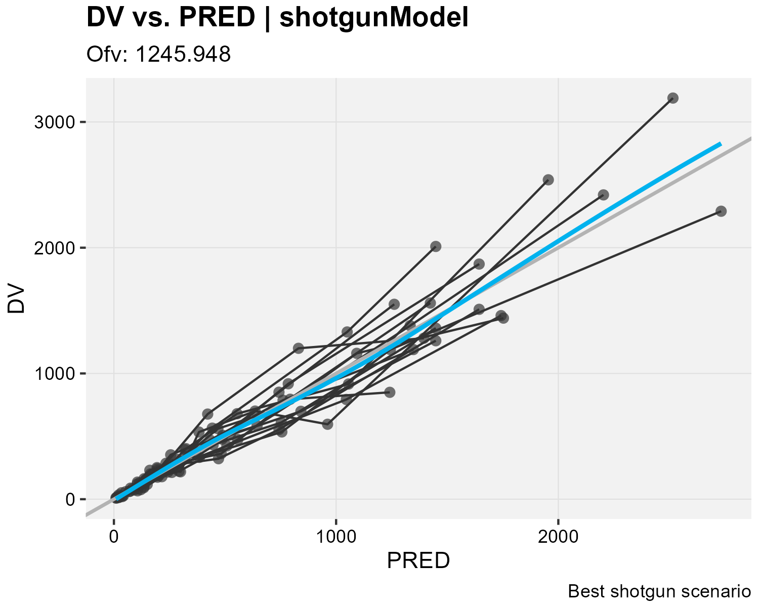
Appendix
listSCMRuns() column reference
| Column | Description |
|---|---|
searchType |
"shotgun" or "stepwise"
|
SCMFolder |
Full path to the timestamped archive folder |
runFolder |
Full path to the individual scenario subfolder |
Scenario |
Human-readable scenario label |
enableFlags |
Comma-separated enable IDs active in this scenario |
status |
"SUCCESS", or another engine status such
as "FAILED"
|
timestamp |
When the SCM run was created |
runId |
Unique identifier for the SCM run |
overallFile |
Path to Overall.csv (if present) |
stepwiseFile |
Path to Stepwise.txt (stepwise runs
only) |
SCMFolder is the top-level archive created by one
invocation of shotgunSearch() or
stepwiseSearch(). runFolder is one scenario
subfolder inside it, containing the NLME fit artifacts for that single
scenario.
Remote host note
When running SCM on a remote Linux host the archive workflow is
transparent. The NLME engine produces a .tar.gz bundle on
the remote server, which Certara.RsNLME downloads and
extracts into the local working directory. After extraction,
listSCMRuns() and getSCMResults() work
identically to local runs.
remoteHost <- hostParams(
  hostType = "RHEL",
  sharedDirectory = "/remote/shared/dir/",
  installationDirectory = "/remote/nlme/install/",
  machineName = "remote.server.example.com",
  parallelMethod = "Multicore",
  numCores = 4,
  userName = "username",
  userPassword = "password",
  rLocation = "/usr/bin",
  isLocal = FALSE
)

shotgunResult <- shotgunSearch(
  model = shotgunModel,
  hostPlatform = remoteHost,
  covariateModel = covariateModel(shotgunModel)
)

allRuns <- listSCMRuns(shotgunResult)
res <- getSCMResults(shotgunResult)
xp <- xposeNlmeModel(model = res$model,
                      fitmodelOutput = res$fitmodelOutput)
Replace the placeholder values in
hostParams()with your actual server credentials and paths. Never store real passwords in scripts; consider using environment variables or a credential manager.