Models with BQL Data • Certara.RsNLME

The purpose of this vignette is to demonstrate how to work with models with Below Quantification Limit (BQL) data using the Certara.RsNLME package, for both built-in and textual PML models.

In this vignette you will:

Use the built-in Certara.RsNLME::pkData dataset to explore syntax for handling BQL data
Create a 2-compartment PK model incorporating BQL data
Explore the different BQL methods available in NLME e.g., static LLOQ vs dataset driven BQL values
Fit the model and perform a Visual Predictive Check (VPC)
Explore censored VPC results using tidyvpc

library(Certara.RsNLME)
library(dplyr)
library(tidyvpc)

Technical Background: BQL and the M3 Method

Below Quantification Limit (BQL) data arises when the true value is unknown but the observed value falls below the assay’s Limit of Quantification (LOQ or LLOQ). In these cases, the observation is censored rather than missing: we know the observed value lies in the interval $(-\infty, \text{LOQ}]$ , but we do not know (and in general never know) the true concentration.

NLME handles censored BQL observations using the M3 method¹. BQL handling is supported within the following estimation methods: Laplacian (Default), Naive Pooled, QRPEM, or IT2S-EM. See the method argument in the engineParams() function for more details.

If a sample is Quantifiable (not BQL), the engine uses the standard Probability Density Function (PDF) implied by the residual error model evaluated at the observed concentration.
If a sample is Censored (BQL), the engine computes the probability (likelihood) that the prediction plus residual error falls below the specified LOQ, i.e., the cumulative probability up to the LOQ rather than the PDF at a single point.

In PML, BQL handling is activated by adding the bql option to the observe statement. There are two main modes:

Dynamic BQL (Dataset-Driven)
The censoring status and LOQ value are taken from the input dataset:
```
error(CEps = 0.1)
// 'bql' keyword activates M3 method
observe(CObs = C * (1 + CEps), bql)
```
and the column mapping associates both the observation and the BQL flag:
```
// Map the observation and the BQL flag column
obs(CObs <- DV, bql <- BQL_Flag)
```
- When BQL_Flag = 0, DV contains the measured concentration.
- When BQL_Flag != 0, DV contains the LLOQ value for that particular sample, and the engine integrates the likelihood from $(-\infty, \text{LLOQ}]$ .
Static BQL (Model-Driven)
The LOQ is hard-coded in the model pml code:
```
error(CEps = 0.1)
// Any DV <= 0.05 is treated as BQL
observe(CObs = C * (1 + CEps), bql = 0.05)
```
In this case, any observation value $\le$ the specified constant (0.05 in above example) is treated as BQL. If both a static value and a BQL flag column are provided, the flag mapping takes precedence. Note that, in general, labs will decline to report any value for BQL samples, and so the data manager may need to provide that value.

The Certara.RsNLME interface (for example through pkmodel() and residualError()) ultimately generates these PML observe(..., bql) or observe(..., bql = <value>) statements for you. If editing PML statements directly, either through editModel or the textualmodel functions, you will need to add the bql term and optional static LLOQ value to the observe() statement. If using dataset-driven BQL, you will need to additionally map the BQL flag column to the BQL model variable using the colMapping() function (details to follow).

Dynamic BQL (Dataset-Driven)

In NLME, BQL information is typically provided via a flag column and an observation column that may contain either a measured value or a sample‑specific LLOQ:

BQL_Flag (or similar): 0 (or blank) = quantifiable, non-zero = BQL.
Observation column (e.g., DV or Conc):
- When BQL_Flag = 0: contains the observed concentration.
- When BQL_Flag != 0: contains the LLOQ value for that record.

This allows the engine to apply the M3 method using the appropriate LOQ for each censored record.

In this vignette, we will demonstrate usage of BQL data by editing the built-in Certara.RsNLME::pkData dataset to include a BQL flag, assigning the lower 20% of Conc values in the data as BQL for illustration.

pk_data_bql <- pkData %>%
  mutate(LLOQ = quantile(Conc, 0.2)) %>%
  mutate(BQL = if_else(Conc < LLOQ, 1, 0)) %>%
  mutate(Conc = if_else(BQL==1, LLOQ, Conc))

In a typical ADaM-style analysis dataset, you can think of the required columns as:

DV: observed concentration (or, for censored records, the LLOQ).
LLOQ: optional explicit lower limit of quantification column (often used in reporting or VPCs).
BQL (or BLQ): flag indicating which records are censored.

We’ll begin by creating the same PK model as before using the pkmodel() function, except this time we’ll include our column mapping arguments and specified data directly in the pkmodel() function.

model_bql <-
  pkmodel(
    numCompartments = 2,
    data = pk_data_bql,
    id = "Subject",
    time = "Act_Time",
    A1 = "Amount",
    CObs = "Conc",
    modelName = "model_bql"
  ) %>%
  structuralParameter(paramName = "V2", hasRandomEffect = FALSE) %>%
  fixedEffect(effect = c("tvV", "tvCl", "tvV2", "tvCl2"),
              value = c(15, 5, 40, 15)) %>%
  randomEffect(effect = c("nV", "nCl", "nCl2"),
               value = rep(0.1, 3))

Use the residualError() function to add dynamic BQL column in the data, we’ll set isBQL = TRUE and the column mapping argument CObsBQL = "CObsBQL", this can also be done at later time using the colMapping() function.

model_bql <- model_bql %>%
  residualError(predName = "C", SD = 0.2, isBQL = TRUE)
#> Warning in residualError(., predName = "C", SD = 0.2, isBQL = TRUE): missing
#> `CObsBQL` argument for model parameterization 'Micro' or 'Clearance'
#> Warning in .map_BQL(.Object, predName, predNameValue = "C", isBQL, mappedBQLcol
#> = CObsBQL, : 'staticLLOQ' argument not provided, specify' CObsBQL' using
#> `colMapping()`

We can see from the warnings above that we could have either specified the staticLLOQ argument, or, if our BQL flag was named CObsBQL in the data, used the argument CObsBQL = "CObsBQL" within residualError(). We’ll proceed to map the CObsBQL model variable to the “BQL” column in the data using the colMapping() function. below.

print(model_bql)
#> 
#>  Model Overview 
#>  ------------------------------------------- 
#> Model Name        :  model_bql
#> Working Directory :  C:/Repos/R-RsNLME/vignettes/model_bql
#> Is population     :  TRUE
#> Model Type        :  PK
#> 
#>  PK 
#>  ------------------------------------------- 
#> Parameterization  :  Clearance
#> Absorption        :  Intravenous
#> Num Compartments  :  2
#> Dose Tlag?        :  FALSE
#> Elimination Comp ?:  FALSE
#> Infusion Allowed ?:  FALSE
#> Sequential        :  FALSE
#> Freeze PK         :  FALSE
#> 
#>  PML 
#>  ------------------------------------------- 
#> test(){
#>     cfMicro(A1,Cl/V, Cl2/V, Cl2/V2)
#>     dosepoint(A1)
#>     C = A1 / V
#>     error(CEps=0.2)
#>     observe(CObs=C * ( 1 + CEps), bql)
#>     stparm(V = tvV * exp(nV))
#>     stparm(Cl = tvCl * exp(nCl))
#>     stparm(V2 = tvV2)
#>     stparm(Cl2 = tvCl2 * exp(nCl2))
#>     fixef( tvV = c(,15,))
#>     fixef( tvCl = c(,5,))
#>     fixef( tvV2 = c(,40,))
#>     fixef( tvCl2 = c(,15,))
#>     ranef(diag(nV,nCl,nCl2) = c(0.1,0.1,0.1))
#> }
#> 
#>  Structural Parameters 
#>  ------------------------------------------- 
#>  V Cl V2 Cl2
#>  ------------------------------------------- 
#> Observations:
#> Observation Name :  CObs
#> Effect Name      :  C
#> Epsilon Name     :  CEps
#> Epsilon Type     :  Multiplicative
#> Epsilon frozen   :  FALSE
#> is BQL           :  TRUE
#>  ------------------------------------------- 
#>  Column Mappings 
#>  ------------------------------------------- 
#> Model Variable Name : Data Column name
#> id                  : Subject
#> time                : Act_Time
#> A1                  : Amount
#> CObs                : Conc
#> CObsBQL             : ?

Something to first point out regarding variable naming conventions, we can see when printing the model that the bql text has been added within the observe() statement.

observe(CObs=C * ( 1 + CEps), bql)

For PK models, the variable name convention in PML for observed concentration is CObs and for the observed effect in PD/Emax models, EObs.

Since the built-in model functions (e.g., pkmodel()) uses default variable naming conventions, we see that CObsBQL is available for mapping.

When the bql term is present inside the observe() statement of the model, the model variable name required for mapping will be {ObsName}BQL e.g., CObsBQL.

 ------------------------------------------- 
 Column Mappings 
 ------------------------------------------- 
...
CObsBQL             : ?

We’ll use the colMapping() function to map CObsBQL model variable to the “BQL” column in the data.

model_bql <- model_bql %>%
  colMapping(c(
    CObsBQL = "BQL"
  ))

Note: The residualError() function can only be used on built-in models. Details for textual models are below.

results_bql <- fitmodel(model_bql)
#> Using MPI host with 4 cores
#> 
#> NLME Job
#> sharedDirectory is not given in the host class instance.
#> Valid NLME_ROOT_DIRECTORY is not given, using current working directory:
#> C:/Repos/R-RsNLME/vignettes
#> TDL5 version: 25.7.1.1
#> 
#> Status: OK
#> License expires: 2026-12-04
#> Refresh until: 2026-01-03 13:09:01
#> Current Date: 2025-12-05
#> The model compiled
#> 
#> Trying to generate job results...
#> Done generating job results.

Copy model, accept parameter estimates.

model_bql_vpc <- copyModel(model_bql, acceptAllEffects = TRUE, modelName = "model_bql_vpc")

Perform a VPC run using the vpcmodel function.

results_bql_vpc <- vpcmodel(model_bql_vpc)
#> Using localhost without parallelization.
#> 
#> NLME Job
#> sharedDirectory is not given in the host class instance.
#> Valid NLME_ROOT_DIRECTORY is not given, using current working directory:
#> C:/Repos/R-RsNLME/vignettes
#> TDL5 version: 25.7.1.1
#> 
#> Status: OK
#> License expires: 2026-12-04
#> Refresh until: 2026-01-03 13:09:01
#> Current Date: 2025-12-05
#> The model compiled
#> 
#> Trying to generate job results...
#> Done generating job results.
#> 
#> VPC/Simulation results are ready in C:/Repos/R-RsNLME/vignettes/model_bql_vpc
#> Loading the results
#> Loading predcheck_bql.csv
#> Loading predcheck0.csv
#> Loading predcheck0_cat.csv
#> Loading predcheck1.csv
#> Loading predcheck1_cat.csv
#> Loading predcheck2.csv
#> Loading predcheck2_cat.csv
#> Loading predout.csv

Extract the observed and simulated data from the vpcmodel() output for use with tidyvpc.

obs_data_bql <- results_bql_vpc$predcheck0

sim_data_bql <- results_bql_vpc$predout

We can see that our resulting VPC data.frame obs_data_bql contains an LLOQ column, we can use this directly in tidyvpc.

dplyr::glimpse(obs_data_bql %>% filter(!is.na(LLOQ)))
#> Rows: 23
#> Columns: 13
#> $ Strat1  <int> 0, 0, 0, 0, 0, 0, 0, 0, 0, 0, 0, 0, 0, 0, 0, 0, 0, 0, 0, 0, 0,…
#> $ Strat2  <int> 0, 0, 0, 0, 0, 0, 0, 0, 0, 0, 0, 0, 0, 0, 0, 0, 0, 0, 0, 0, 0,…
#> $ Strat3  <int> 0, 0, 0, 0, 0, 0, 0, 0, 0, 0, 0, 0, 0, 0, 0, 0, 0, 0, 0, 0, 0,…
#> $ ID1     <lgl> NA, NA, NA, NA, NA, NA, NA, NA, NA, NA, NA, NA, NA, NA, NA, NA…
#> $ ID2     <lgl> NA, NA, NA, NA, NA, NA, NA, NA, NA, NA, NA, NA, NA, NA, NA, NA…
#> $ ID3     <lgl> NA, NA, NA, NA, NA, NA, NA, NA, NA, NA, NA, NA, NA, NA, NA, NA…
#> $ ID4     <lgl> NA, NA, NA, NA, NA, NA, NA, NA, NA, NA, NA, NA, NA, NA, NA, NA…
#> $ ID5     <int> 1, 2, 2, 3, 4, 4, 5, 6, 6, 6, 7, 7, 8, 9, 9, 10, 11, 11, 13, 1…
#> $ IVAR    <dbl> 23.78, 8.11, 24.08, 23.95, 8.12, 23.90, 23.94, 4.01, 8.03, 24.…
#> $ DV      <chr> "BLOQ", "BLOQ", "BLOQ", "BLOQ", "BLOQ", "BLOQ", "BLOQ", "BLOQ"…
#> $ LLOQ    <dbl> 102.4, 102.4, 102.4, 102.4, 102.4, 102.4, 102.4, 102.4, 102.4,…
#> $ ObsName <chr> "CObs", "CObs", "CObs", "CObs", "CObs", "CObs", "CObs", "CObs"…
#> $ Reset   <int> 0, 0, 0, 0, 0, 0, 0, 0, 0, 0, 0, 0, 0, 0, 0, 0, 0, 0, 0, 0, 0,…

Next, we’ll do a little bit of data cleaning to prepare the data for use with tidyvpc.

Note, it is necessary to coerce the DV column to numeric before using it in tidyvpc. NLME returns the text “BLOQ” in the DV column, we can convert this to -Inf. Additionally, the LLOQ column is NA where DV != "BLOQ" so we’ll replace the NA values with -Inf as well.

obs_data_bql$DV <- as.numeric(obs_data_bql$DV)
obs_data_bql <- obs_data_bql %>%
  mutate(DV = if_else(is.na(DV), -Inf, DV)) %>%
  mutate(LLOQ = if_else(is.na(LLOQ), -Inf, LLOQ))

At this point, the obs_data_bql object contains:

DV: numeric, with BLOQ rows set to -Inf.
LLOQ: numeric, with non-BLOQ rows set to -Inf.

This structure makes it straightforward to define the BQL indicator for tidyvpc::censoring() using a simple logical expression DV < LLOQ. Recall from the tidyvpc documentation that:

blq must be a logical vector (no NA values) indicating whether each observation is below the LLOQ.
lloq must be a numeric vector giving the limit for those BLQ rows.

The call

censoring(blq = (DV < LLOQ), lloq = LLOQ)

therefore tells tidyvpc to:

mark records with DV < LLOQ as BLQ,
use the corresponding LLOQ value as the limit,
and compute the percentage of BLQ observations per bin when plot(vpc, censoring.type = "blq") is used.

Generate censored VPC using tidyvpc. See here for additional details.

vpc_bql <- observed(obs_data_bql, x=IVAR, y=DV) %>%
    simulated(sim_data_bql, y=DV) %>%
    censoring(blq=(DV < LLOQ), lloq=LLOQ) %>%
    binning(bin = "jenks", nbins = 5) %>%
    vpcstats()

Combined plot showing VPC and Percentage of BQL.

plot(vpc_bql, censoring.type = "blq")
#> Warning: Removed 4 rows containing missing values or values outside the scale range
#> (`geom_line()`).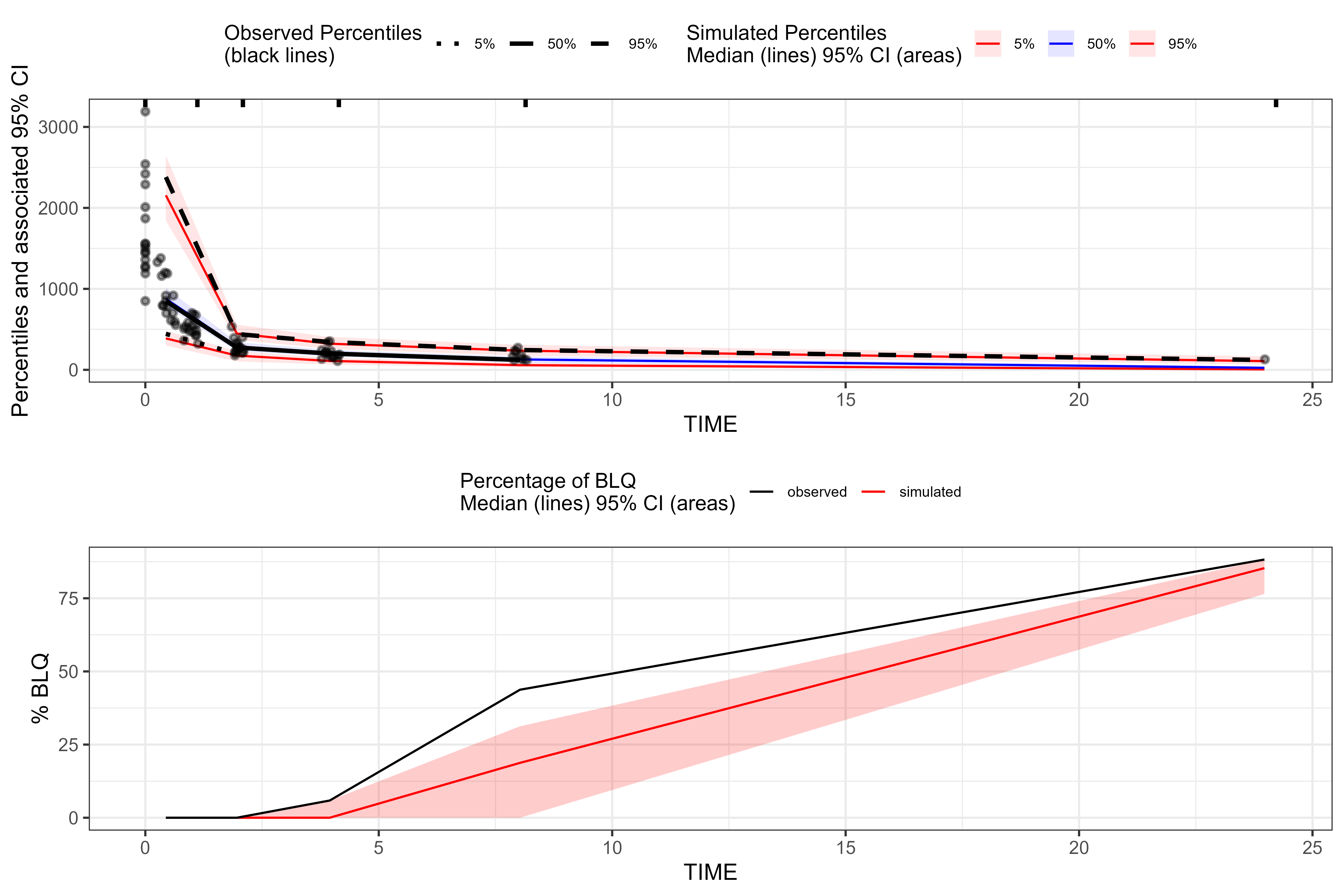

View BQL data at lower concentrations using coord_cartesian() from ggplot2.

library(ggplot2)

plot(vpc_bql) + coord_cartesian(ylim = c(0, 1000))

Static BQL / Static LLOQ

In some studies, the LOQ is constant (e.g., a single assay with a fixed LLOQ across all samples). In these cases, it can be convenient to specify a single static LLOQ in the model rather than carrying a BQL flag and sample-specific LLOQ values in the dataset.

In PML, this corresponds to using a numeric argument on the bql option:

error(CEps = 0.1)
// Any DV <= 0.05 is treated as BQL
observe(CObs = C * (1 + CEps), bql = 0.05)

In Certara.RsNLME, the same idea is exposed through the staticLLOQ argument on residualError(). You still indicate that the model has BQL data using isBQL = TRUE, but you do not need to map a BQL flag column when a static LLOQ is sufficient.

static_lloq_value <- 50

model_bql_static <-
  pkmodel(
    numCompartments = 2,
    data = pkData,
    id = "Subject",
    time = "Act_Time",
    A1 = "Amount",
    CObs = "Conc",
    modelName = "model_bql_static"
  ) %>%
  structuralParameter(paramName = "V2", hasRandomEffect = FALSE) %>%
  fixedEffect(
    effect = c("tvV", "tvCl", "tvV2", "tvCl2"),
    value = c(15, 5, 40, 15)
  ) %>%
  randomEffect(
    effect = c("nV", "nCl", "nCl2"),
    value = rep(0.1, 3)
  ) %>%
  residualError(
    predName = "C",
    SD = 0.2,
    isBQL = TRUE,
    staticLLOQ = static_lloq_value
  )

Here, any observation mapped to CObs with value $\le$ static_lloq_value is treated as BQL in the likelihood calculation. No additional CObsBQL mapping is required, although you may still choose to carry an explicit BQL flag column in your dataset for reporting or diagnostics.

We can now fit the model and generate a VPC in exactly the same way as before:

results_bql_static <- fitmodel(model_bql_static)
#> Using MPI host with 4 cores
#> 
#> NLME Job
#> sharedDirectory is not given in the host class instance.
#> Valid NLME_ROOT_DIRECTORY is not given, using current working directory:
#> C:/Repos/R-RsNLME/vignettes
#> TDL5 version: 25.7.1.1
#> 
#> Status: OK
#> License expires: 2026-12-04
#> Refresh until: 2026-01-03 13:09:01
#> Current Date: 2025-12-05
#> The model compiled
#> 
#> Trying to generate job results...
#> Done generating job results.

model_bql_static_vpc <-
  copyModel(
    model_bql_static,
    acceptAllEffects = TRUE,
    modelName = "model_bql_static_vpc"
  )

results_bql_static_vpc <- vpcmodel(model_bql_static_vpc)
#> Using localhost without parallelization.
#> 
#> NLME Job
#> sharedDirectory is not given in the host class instance.
#> Valid NLME_ROOT_DIRECTORY is not given, using current working directory:
#> C:/Repos/R-RsNLME/vignettes
#> TDL5 version: 25.7.1.1
#> 
#> Status: OK
#> License expires: 2026-12-04
#> Refresh until: 2026-01-03 13:09:01
#> Current Date: 2025-12-05
#> The model compiled
#> 
#> Trying to generate job results...
#> Done generating job results.
#> 
#> VPC/Simulation results are ready in C:/Repos/R-RsNLME/vignettes/model_bql_static_vpc
#> Loading the results
#> Loading predcheck_bql.csv
#> Loading predcheck0.csv
#> Loading predcheck0_cat.csv
#> Loading predcheck1.csv
#> Loading predcheck1_cat.csv
#> Loading predcheck2.csv
#> Loading predcheck2_cat.csv
#> Loading predout.csv

Extract the observed and simulated data for use with tidyvpc:

obs_data_bql_static <- results_bql_static_vpc$predcheck0
sim_data_bql_static <- results_bql_static_vpc$predout

As in the dynamic BQL example, the obs_data_bql_static data.frame contains an LLOQ column that can be used directly with tidyvpc and other tools. The DV column will contain "BLOQ" for censored records, which can be converted to numeric values and handled using the same strategy shown above for obs_data_bql.

obs_data_bql_static$DV <- as.numeric(obs_data_bql_static$DV)
obs_data_bql_static <- obs_data_bql_static %>%
  mutate(DV = if_else(is.na(DV), -Inf, DV)) %>%
  mutate(LLOQ = if_else(is.na(LLOQ), -Inf, LLOQ))

vpc_bql_static <- observed(obs_data_bql_static, x = IVAR, y = DV) %>%
  simulated(sim_data_bql_static, y = DV) %>%
  censoring(blq = (DV < LLOQ), lloq = LLOQ) %>%
  binning(bin = "jenks", nbins = 5) %>%
  vpcstats()

plot(vpc_bql_static, censoring.type = "blq")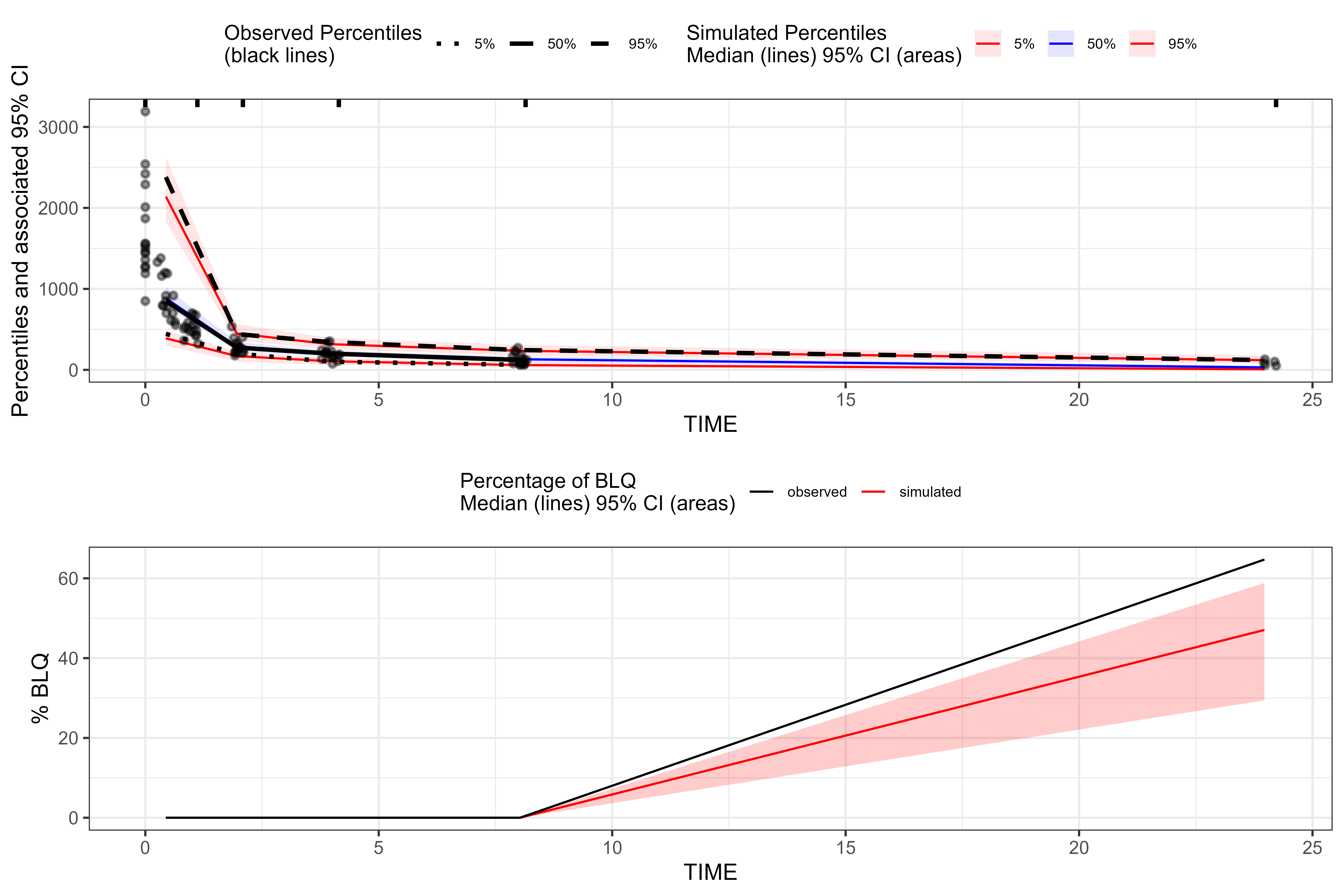

From tidyvpc’s perspective, the dynamic-BQL and static-LLOQ workflows look identical: both supply a numeric LLOQ column and use DV < LLOQ to define the BLQ indicator passed to censoring(). The difference lies upstream in how NLME generates the BQL information (dataset‑driven flag vs constant LLOQ) and how that censoring mechanism relates to the study design.

When both a BQL flag mapping (e.g., CObsBQL) and a staticLLOQ value are provided to residualError(), the flag mapping takes precedence for determining which records are censored, consistent with the underlying PML behavior described in the knowledge base.

Comparing Censored vs Traditional VPC

In the code below, we’ll fit the same model as above, but without the BQL data.

model_no_bql <-
  pkmodel(numCompartments = 2,
          columnMap = FALSE,
          modelName = "model_no_bql") %>%
  structuralParameter(paramName = "V2", hasRandomEffect = FALSE) %>%
  fixedEffect(effect = c("tvV", "tvCl", "tvV2", "tvCl2"),
              value = c(15, 5, 40, 15)) %>%
  randomEffect(effect = c("nV", "nCl", "nCl2"),
               value = rep(0.1, 3)) %>%
  residualError(predName = "C", SD = 0.2) %>%
  dataMapping(pkData) %>%
  colMapping(c(
    id = "Subject",
    time = "Act_Time",
    A1 = "Amount",
    CObs = "Conc"
  ))

results_no_bql <- fitmodel(model_no_bql)
#> Using MPI host with 4 cores
#> 
#> NLME Job
#> sharedDirectory is not given in the host class instance.
#> Valid NLME_ROOT_DIRECTORY is not given, using current working directory:
#> C:/Repos/R-RsNLME/vignettes
#> TDL5 version: 25.7.1.1
#> 
#> Status: OK
#> License expires: 2026-12-04
#> Refresh until: 2026-01-03 13:09:01
#> Current Date: 2025-12-05
#> The model compiled
#> 
#> Trying to generate job results...
#> Done generating job results.

model_no_bql_vpc <- copyModel(model_no_bql, acceptAllEffects = TRUE, modelName = "model_no_bql_vpc")

results_no_bql_vpc <- vpcmodel(model_no_bql_vpc)
#> Using localhost without parallelization.
#> 
#> NLME Job
#> sharedDirectory is not given in the host class instance.
#> Valid NLME_ROOT_DIRECTORY is not given, using current working directory:
#> C:/Repos/R-RsNLME/vignettes
#> TDL5 version: 25.7.1.1
#> 
#> Status: OK
#> License expires: 2026-12-04
#> Refresh until: 2026-01-03 13:09:01
#> Current Date: 2025-12-05
#> The model compiled
#> 
#> Trying to generate job results...
#> Done generating job results.
#> 
#> VPC/Simulation results are ready in C:/Repos/R-RsNLME/vignettes/model_no_bql_vpc
#> Loading the results
#> Loading predcheck_bql.csv
#> Loading predcheck0.csv
#> Loading predcheck0_cat.csv
#> Loading predcheck1.csv
#> Loading predcheck1_cat.csv
#> Loading predcheck2.csv
#> Loading predcheck2_cat.csv
#> Loading predout.csv

obs_data_no_bql <- results_no_bql_vpc$predcheck0

sim_data_no_bql <- results_no_bql_vpc$predout

Generate VPC using tidyvpc for the model without BQL data.

vpc_no_bql <- observed(obs_data_no_bql, x=IVAR, y=DV) %>%
    simulated(sim_data_no_bql, y=DV) %>%
    binning(bin = "jenks", nbins = 5) %>%
    vpcstats()

Compare the two VPCs using the grid.arrange() function from the gridExtra package.

library(gridExtra)
#> 
#> Attaching package: 'gridExtra'
#> The following object is masked from 'package:dplyr':
#> 
#>     combine
p1 <- plot(vpc_no_bql) + coord_cartesian(ylim = c(0, 1000))
p2 <- plot(vpc_bql_static) + coord_cartesian(ylim = c(0, 1000)) + geom_hline(yintercept = static_lloq_value, linetype = "dotted")

grid.arrange(p1, p2, nrow = 2)
#> Warning: Removed 2 rows containing missing values or values outside the scale range
#> (`geom_line()`).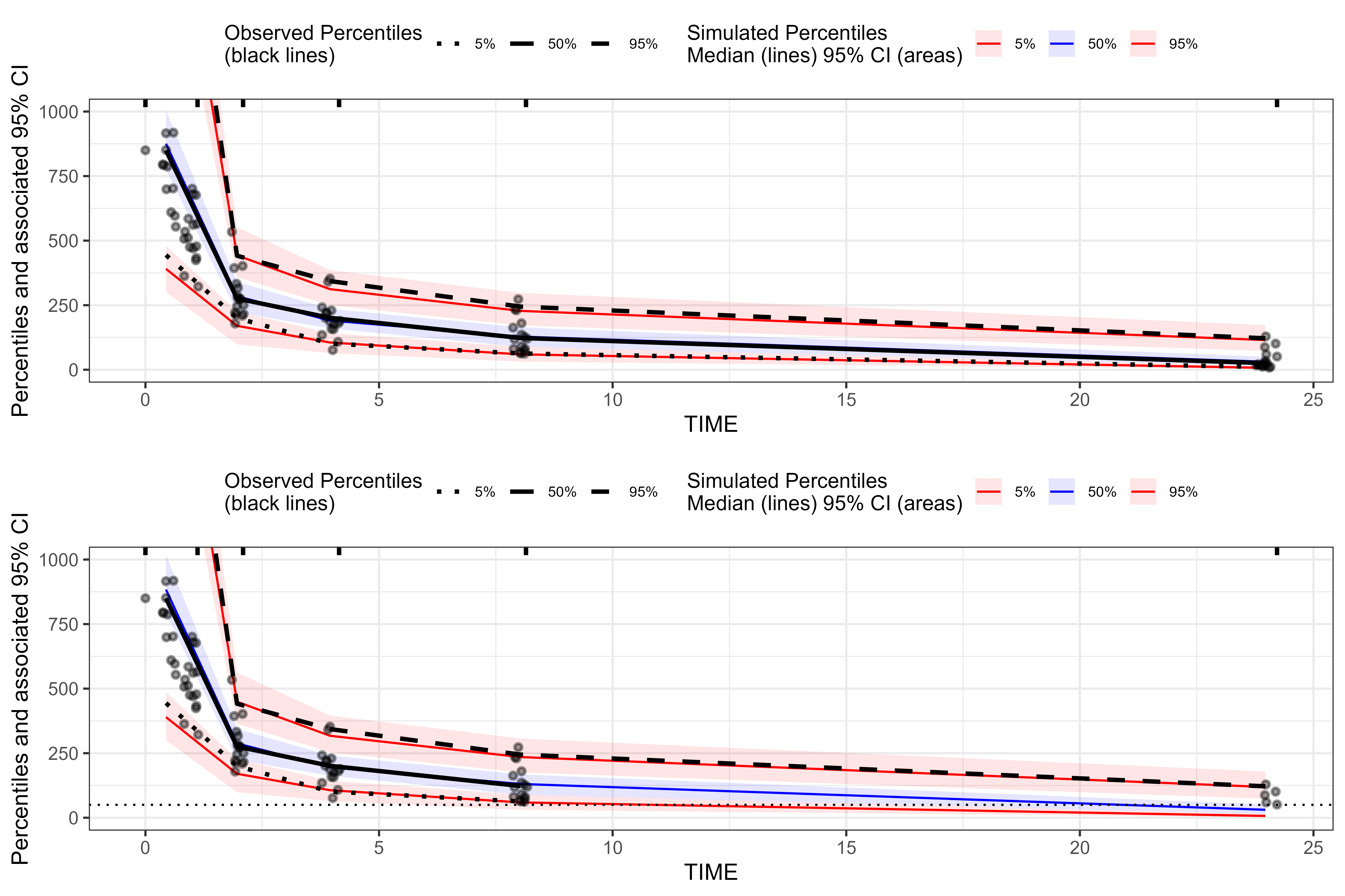

In the traditional VPC (top), all observed data points and observed percentile lines are shown, even when concentrations fall well below the assay LLOQ. In the censored VPC with censoring() (bottom), tidyvpc uses the blq and lloq information to suppress observed percentiles and points below the LLOQ. As a result, the lower observed percentile line is truncated at the horizontal dotted line (the LLOQ of static_lloq_value), and no black points are drawn underneath it. This behavior reflects the fact that, for BLQ samples, we only know that the true value lies somewhere below the LLOQ; tidyvpc therefore does not plot pseudo‑exact observed concentrations below that limit when a censored VPC is requested.