Using Model Results with RsNLME

Overview

The Certara.ModelResults Shiny GUI and script generating functionality can be used alongside Certara.RsNLME for a robust, efficient, and reproducible pharmacometric modeling workflow in R.

Users can iterate over multiple models in R, and easily pass the model output files to Certara.ModelResults to generate model diagnostic plots and tables in the Shiny GUI. Furthermore, all plots and tables generated in the Shiny GUI include the associated R and/or Rmd code to reproduce the model diagnostics from the command line in R.

Build and execute models in RsNLME and launch the Shiny GUI with model objects

We’ll first need to build and execute our models using the Certara.RsNLME package. We will be using the example data file pkData from the Certara.RsNLME package.

Build base model

We’ll define a basic two-compartment population PK model with IV bolus (through the Certara.RsNLME built-in function pkmodel()) as well as its associated column mappings. Help is available by typing ?Certara.RsNLME::pkmodel.

Note: The corresponding R script used in this example can be found in RsNLME_Examples/TwoCptIVBolus_FitBaseModel_CovariateSearch_VPC_BootStrapping.R. RsNLME Example Scripts

library(Certara.RsNLME)
library(magrittr)

baseModel <- pkmodel(numCompartments = 2, data = pkData,
                    ID = "Subject", Time = "Act_Time", A1 = "Amount", CObs = "Conc", 
                    modelName = "TwCpt_IVBolus_FOCE_ELS")

Next, we’ll update parameters in our pkmodel:

Disable the corresponding random effects for structural parameter V2
Change initial values for fixed effects, tvV, tvCl, tvV2, and tvCl2, to be 15, 5, 40, and 15, respectively
Change the covariance matrix of random effects, nV, nCl, and nCl2, to be a diagonal matrix with all its diagonal elements being 0.1
Change the standard deviation of residual error to be 0.2

baseModel <- baseModel %>%
  structuralParameter(paramName = "V2", hasRandomEffect = FALSE) %>%
  fixedEffect(effect = c("tvV", "tvCl", "tvV2", "tvCl2"), value = c(15, 5, 40, 15)) %>%
  randomEffect(effects = c("nV", "nCl", "nCl2"), values = rep(0.1, 3)) %>%
  residualError(predName = "C", SD = 0.2)

Fit the base model

Fit the model using the default host and default values for the relevant NLME engine arguments. For this example model, FOCE-ELS is the default method for estimation, and Sandwich is the default method for standard error calculations.

Note: The default values for the relevant NLME engine arguments are chosen based on the model, type ?Certara.RsNLME::engineParams for details.

baseFitJob <- fitmodel(baseModel)

Launch `resultsUI()` with base model

The model argument in resultsUI() can be supplied as either a single model object or a vector of model objects or a list of model objects. We can now provide our model object, baseModel, to the model argument in resultsUI() and execute Model Results.

library(Certara.ModelResults)

resultsUI(model = baseModel)

The series of screenshots below demonstrate how users can preview model diagnostic plots and tables using the tree selection in the Shiny GUI.

Build covariate model

We will copy our baseModel and accept parameter estimates before adding a covariate in the next step.

covariateModel <- copyModel(baseModel, 
                          acceptAllEffects = TRUE, 
                          modelName = "TwCpt_IVBolus_SelectedCovariateModel_FOCE_ELS")

Next, we’ll add the continuous covariate BodyWeight to our model and set the covariate effect on structural parameters V and Cl.

covariateModel <- covariateModel %>%
  addCovariate(covariate = "BodyWeight", effect = c("V", "Cl"))

Fit the covariate model

covariateFitJob <- fitmodel(covariateModel)

Launch `resultsUI()` with multiple models

Finally, we can supply a vector of model objects to the model argument in resultsUI() and execute Model Results.

library(Certara.ModelResults)

resultsUI(model = c(baseModel, covariateModel))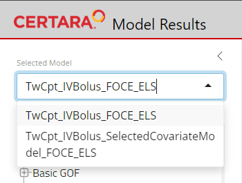

rsnlme-mult-mods

Advanced Examples

Below are a few examples of advanced modeling use cases that are easily achieved with RsNLME + Model Results.

Example 1: Looping through model scenarios

We can use different numbers of compartments to loop through multiple model scenarios in the following code, then easily pass the models to resultsUI()

library(Certara.RsNLME)
# Setup compartment scenarios
numCpt <-  c(1, 2, 3)
namesCpt <-  c("OneCpt", "TwoCpt", "ThreeCpt")
numScenarios <- length(numCpt)

# Memory allocation for model objects
models <- vector(mode = "list", length = numScenarios)
names(models) <- namesCpt

# Memory allocation for job objects
jobs <- vector(mode = "list", length = numScenarios)
names(jobs) <- namesCpt

# Define models and then run them 
for (i in 1:numScenarios){

  ## Define a basic PK model with IV Bolus as well as the associated column mapping
  models[[i]] <- pkmodel(numCompartments = numCpt[i],
                        ID = "Subject", Time = "Act_Time", A1 = "Amount", CObs = "Conc",
                        data = pkData, modelName = paste0(namesCpt[i], "_IVBolus_FOCE-ELS")) %>%
                fixedEffect(effect = "tvV", value = 5)  # Set initial value for theta to 5
  ## Fit model
  jobs[[i]] <- fitmodel(models[[i]])
}

Execute resultsUI() with our compartment scenario models:

library(Certara.ModelResults)

resultsUI(model = models)

Example 2: Using PML (.mdl file)

Import data

dataPath <- system.file("extdata","PKCategoricalData.csv",package="Certara.ModelResults")

pkCategoricalData <- read.csv(dataPath)

head(pkCategoricalData)
#>   ID Time Dose      CObs CategoricalObs
#> 1  1  0.0   10        NA             NA
#> 2  1  0.5   NA 0.5395386              1
#> 3  1  1.0   NA 0.8087664              1
#> 4  1  2.0   NA 1.2350127              0
#> 5  1  4.0   NA 1.1687156              0
#> 6  1  8.0   NA 0.8421397              0

Create textual model

library(Certara.RsNLME)
library(magrittr)

mdlPath <-  system.file("extdata","PKCategorical_OneCpt1stOrderAbsorp_2CategoriesLogitImax.mdl",package="Certara.ModelResults")


model <- textualmodel(modelName = "PKCategorical_OneCpt1stOrderAbsorp_LogitImax", 
                      mdl = mdlPath, 
                      data = pkCategoricalData)

Map columns

We can see in the “Column Mappings” section of the print(model) output that model variable Aa was not automatically mapped, since the corresponding column is named Dose in our dataset. In such cases where the model variable name is different from the column name in the dataset, we will have to manually map.

model <- model %>%
  colMapping(c(Aa = "Dose"))

Fit model

Engine parameters setup:

Set the engine method to be QPREM
Set the number of replicates to generate PCWRES to 1000
Use the default value for all the other relevant arguments

engineSetup <- engineParams(model, method = "QRPEM", numRepPCWRES = 1000)

Run the model.

job <- fitmodel(model, params = engineSetup)

Create `xpose_data` object

Import results of an NLME run into xpose database to create commonly used diagnostic plots.

library(Certara.Xpose.NLME)

xpdb <- xposeNlme(dir = model@modelInfo@workingDir, modelName = "PKCategorical_OneCpt1stOrderAbsorp_LogitImax")

We can exclude observed variables using the xpose::filter() command. Let’s exclude the categorical observed variable, CategoricalObs, from our model diagnostic plots.

library(xpose)

xpdb <- xpdb %>%
  filter(ObsName != "CategoricalObs")

Launch `resultsUI()`

library(Certara.ModelResults)

resultsUI(xpdb = xpdb)