Advanced Plot Customization

Overview

Certara.ModelResults uses functions from both the xpose and Certara.Xpose.NLME packages to generate model diagnostic plots. The resulting class object returned from the plotting functions is a ggplot object however, which means we can use additional functions from the ggplot2 package to further customize our plot.

Combine multiple plots

Tag GOF plots in `resultsUI()`

We can combine separate plots that we’ve generated in resultsUI() into a single plot. To begin, we’ll launch Certara.ModelResults with our example data xpdb_NLME and tag the following Goodness of Fit (GOF) plots: DV vs PRED, DV vs IPRED, CWRES vs PRED, CWRES vs IVAR.

library(Certara.ModelResults)

resultsUI(xpdb = xpdb_NLME)

A gif of multiple GOF plots being tagged and downloaded from the ModelResults Shiny GUI.

Download R script from Shiny GUI

The following R script GOF_plots.R was downloaded from the Shiny GUI.


library(Certara.ModelResults)
library(Certara.Xpose.NLME)
library(xpose)
library(ggplot2)
library(dplyr)
library(tidyr)
library(magrittr)
library(flextable)

xpobj <- xpdb_NLME[["TwCpt_IVBolus_SelectedCovariateModel_FOCE_ELS"]]
plot <- xpobj %>%
  filter(!is.na(ObsName)) %>%
  dv_vs_pred(type = "ps", facets = c("ObsName", NULL), scales = "free", nrow = NULL, ncol = NULL, subtitle = "-2LL: @ofv", page = NULL, guide = TRUE, guide_linetype = "dashed", guide_alpha = 0.5, guide_color = "#000000", guide_linewidth = 1L, smooth_method = "loess", smooth_span = 0.75, smooth_linetype = "solid", smooth_color = "#D63636", smooth_linewidth = 1.2, log = NULL, point_shape = 16, point_color = "#757D8F", point_alpha = 0.5, point_size = 3.9, line_color = "#000000", line_alpha = 0.5, line_linewidth = 1L, line_linetype = "solid") + 
 theme_certara()
plot


xpobj <- xpdb_NLME[["TwCpt_IVBolus_SelectedCovariateModel_FOCE_ELS"]]
plot <- xpobj %>%
  filter(!is.na(ObsName)) %>%
  dv_vs_ipred(type = "ps", facets = c("ObsName", NULL), scales = "free", nrow = NULL, ncol = NULL, page = NULL, subtitle = "-2LL: @ofv, Eps shrink: @epsshk", guide = TRUE, guide_linetype = "dashed", guide_alpha = 0.5, guide_color = "#000000", guide_linewidth = 1L, smooth_method = "loess", smooth_span = 0.75, smooth_linetype = "solid", smooth_color = "#D63636", smooth_linewidth = 1.2, log = NULL, point_shape = 16, point_color = "#757D8F", point_alpha = 0.5, point_size = 3.9, line_color = "#000000", line_alpha = 0.5, line_linewidth = 1L, line_linetype = "solid") + 
 theme_certara()
plot


xpobj <- xpdb_NLME[["TwCpt_IVBolus_SelectedCovariateModel_FOCE_ELS"]]
plot <- xpobj %>%
  filter(!is.na(ObsName)) %>%
  res_vs_pred(res = "CWRES", type = "ps", facets = c("ObsName", NULL), nrow = NULL, ncol = NULL, scales = "free", subtitle = "-2LL: @ofv", page = NULL, smooth_method = "loess", smooth_span = 0.75, smooth_linetype = "solid", smooth_color = "#D63636", smooth_linewidth = 1.2, log = NULL, guide = TRUE, guide_linetype = "dashed", guide_alpha = 0.5, guide_color = "#000000", guide_linewidth = 1L, point_shape = 16, point_color = "#757D8F", point_alpha = 0.5, point_size = 3.9, line_color = "#000000", line_alpha = 0.5, line_linewidth = 1L, line_linetype = "solid") + 
 theme_certara()
plot


xpobj <- xpdb_NLME[["TwCpt_IVBolus_SelectedCovariateModel_FOCE_ELS"]]
plot <- xpobj %>%
  filter(!is.na(ObsName)) %>%
  res_vs_idv(res = "CWRES", type = "ps", facets = c("ObsName", NULL), scales = "free", nrow = NULL, ncol = NULL, subtitle = "-2LL: @ofv", page = NULL, smooth_method = "loess", smooth_span = 0.75, smooth_linetype = "solid", smooth_color = "#D63636", smooth_linewidth = 1.2, log = NULL, guide = TRUE, guide_linetype = "dashed", guide_alpha = 0.5, guide_color = "#000000", guide_linewidth = 1L, point_shape = 16, point_color = "#757D8F", point_alpha = 0.5, point_size = 3.9, line_color = "#000000", line_alpha = 0.5, line_linewidth = 1L, line_linetype = "solid") + 
 theme_certara()
plot

Create plot objects

To combine the individual plots into a single plot, we’ll assign these plots new distinct values: plot_dv_pred, plot_dv_ipred, plot_cwres_pred, plot_cwres_time.

library(Certara.Xpose.NLME)
library(xpose)
library(ggplot2)

xpobj <- xpdb_NLME[["TwCpt_IVBolus_SelectedCovariateModel_FOCE_ELS"]]

plot_dv_pred <- xpobj %>%
  filter(!is.na(ObsName)) %>%
  dv_vs_pred(type = "ps", facets = c("ObsName", NULL), scales = "free", nrow = NULL, ncol = NULL, subtitle = "-2LL: @ofv", page = NULL, guide = TRUE, guide_linetype = "dashed", guide_alpha = 0.5, guide_color = "#000000", guide_linewidth = 1L, smooth_method = "loess", smooth_span = 0.75, smooth_linetype = "solid", smooth_color = "#D63636", smooth_linewidth = 1.2, log = NULL, point_shape = 16, point_color = "#757D8F", point_alpha = 0.5, point_size = 3.9, line_color = "#000000", line_alpha = 0.5, line_linewidth = 1L, line_linetype = "solid") + 
 theme_certara()


plot_dv_ipred <- xpobj %>%
  filter(!is.na(ObsName)) %>%
  dv_vs_ipred(type = "ps", facets = c("ObsName", NULL), scales = "free", nrow = NULL, ncol = NULL, page = NULL, subtitle = "-2LL: @ofv, Eps shrink: @epsshk", guide = TRUE, guide_linetype = "dashed", guide_alpha = 0.5, guide_color = "#000000", guide_linewidth = 1L, smooth_method = "loess", smooth_span = 0.75, smooth_linetype = "solid", smooth_color = "#D63636", smooth_linewidth = 1.2, log = NULL, point_shape = 16, point_color = "#757D8F", point_alpha = 0.5, point_size = 3.9, line_color = "#000000", line_alpha = 0.5, line_linewidth = 1L, line_linetype = "solid") + 
 theme_certara()



plot_cwres_pred <- xpobj %>%
  filter(!is.na(ObsName)) %>%
  res_vs_pred(res = "CWRES", type = "ps", facets = c("ObsName", NULL), nrow = NULL, ncol = NULL, scales = "free", subtitle = "-2LL: @ofv", page = NULL, smooth_method = "loess", smooth_span = 0.75, smooth_linetype = "solid", smooth_color = "#D63636", smooth_linewidth = 1.2, log = NULL, guide = TRUE, guide_linetype = "dashed", guide_alpha = 0.5, guide_color = "#000000", guide_linewidth = 1L, point_shape = 16, point_color = "#757D8F", point_alpha = 0.5, point_size = 3.9, line_color = "#000000", line_alpha = 0.5, line_linewidth = 1L, line_linetype = "solid") + 
 theme_certara()



plot_cwres_time <- xpobj %>%
  filter(!is.na(ObsName)) %>%
  res_vs_idv(res = "CWRES", type = "ps", facets = c("ObsName", NULL), scales = "free", nrow = NULL, ncol = NULL, subtitle = "-2LL: @ofv", page = NULL, smooth_method = "loess", smooth_span = 0.75, smooth_linetype = "solid", smooth_color = "#D63636", smooth_linewidth = 1.2, log = NULL, guide = TRUE, guide_linetype = "dashed", guide_alpha = 0.5, guide_color = "#000000", guide_linewidth = 1L, point_shape = 16, point_color = "#757D8F", point_alpha = 0.5, point_size = 3.9, line_color = "#000000", line_alpha = 0.5, line_linewidth = 1L, line_linetype = "solid") + 
 theme_certara()

Combine plots using `grid.arrange()`

We will use grid.arrange() from the gridExtra package to arrange our plots into a single grid.

Note: I have specified fig.width = 8, fig.height = 8 in the Rmd chunk options to reproduce this plot dimension.

library(gridExtra)

plot_combined_gof <- grid.arrange(plot_dv_pred, plot_dv_ipred, plot_cwres_pred, plot_cwres_time)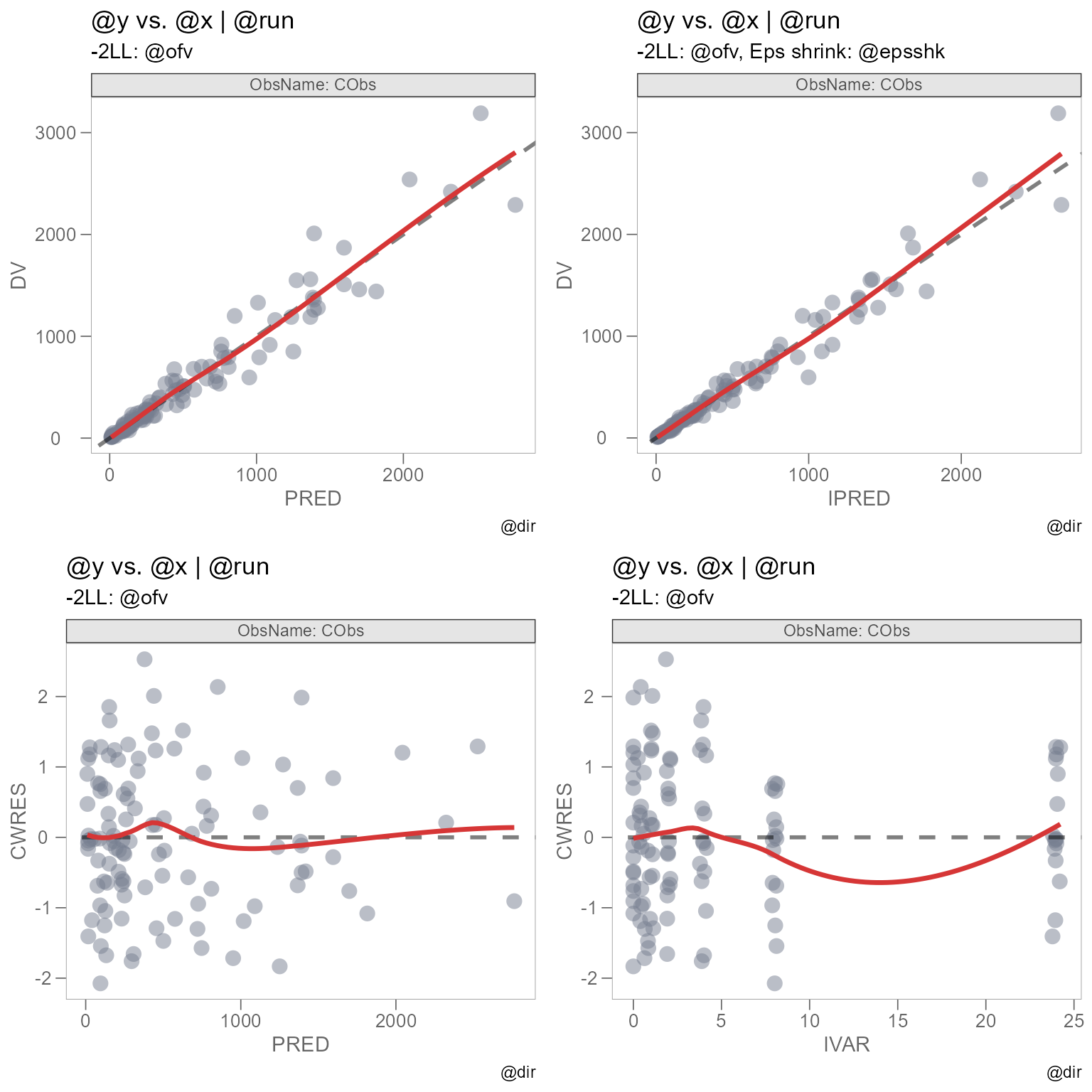

An image of the four individual plots combined into one figure.

We can see that there are some issues with our plot titles. The titles and subtitles originally utilized the @ keyword from the xpose package, which allows us to specify key variables in our xpose_data object as plot text. See template_titles().

However, the functionality offered by template_titles() only works if the plot is of class xpose_plot.

class(plot_dv_pred)
#> [1] "xpose_plot" "gg"         "ggplot"

We can see that our combined GOF plot is of the following classes:

class(plot_combined_gof)
#> [1] "gtable" "gTree"  "grob"   "gDesc"

To resolve the issue with our titles, we’ll manually change the titles of our individual plots, without using the @ tag from template_titles(), since this functionality is not supported. Let’s also remove the subtitle and caption for each plot.

Note: This can be done in the Shiny GUI. Navigate to the “DISPLAY” subtab under the “PREVIEW” tab and uncheck “Default Text” to change text in the GUI, then tag the plot and generate the corresponding R code.


plot_dv_pred <- plot_dv_pred + 
  labs(title = "DV vs PRED", subtitle = NULL, caption = NULL)
  
plot_dv_ipred <- plot_dv_ipred + 
  labs(title = "DV vs IPRED", subtitle = NULL, caption = NULL)

plot_cwres_pred <- plot_cwres_pred + 
  labs(title = "CWRES vs PRED", subtitle = NULL, caption = NULL)

plot_cwres_time <- plot_cwres_time + 
  labs(title = "CWRES vs TIME", subtitle = NULL, caption = NULL)

Now, we’ll arrange our combined GOF plots once again.


plot_combined_gof <- grid.arrange(plot_dv_pred, plot_dv_ipred, plot_cwres_pred, plot_cwres_time)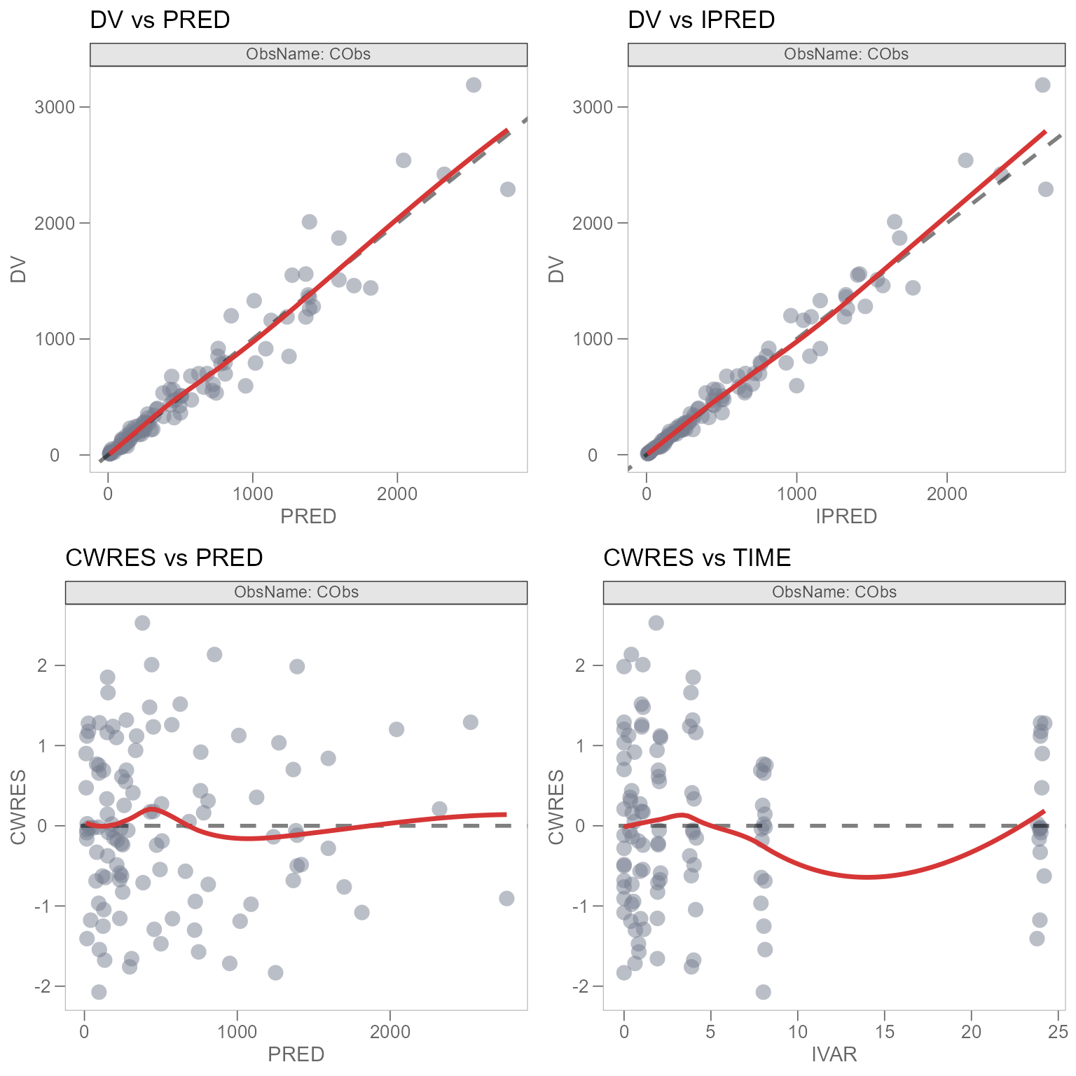

The same four plots with new titles combined into one figure.

Our plot_combined_gof is looking much better now. But what if we want to overlay an additional title and subtitle on the combined GOF plot? We can do so by combining a rectGrob and textGrob() from the grid package.

Using textGrob() can be sufficient on its own in some use cases, but this function is unable to add a background color to the text. This means that a report rendered on a dark mode HTML page for example may be hard to read with the text and background being similar colors. To compensate for this, we can create a container for the text using rectGrob. This will create a rectangular division that we can set to the same width and color as our plot. Within this container, we’ll define a textGrob() for both the title and subtitle. We will extract the ofv and epsshk values contained in our xpobj and define them in the subtitle.

library(grid)
library(gridExtra)
library(dplyr)

ofv <- xpobj$summary %>%
  filter(problem == 1 & label == "ofv") %>%
  select(value)

eps_shk <- xpobj$summary %>%
  filter(problem == 1 & label == "epsshk") %>%
  select(value)

# Title
title_grob <- grobTree(
  rectGrob(width = unit(1, "npc"), gp=gpar(fill = "white", col = NA)), 
  textGrob('GOF Plots for Two Cpt IV Bolus Selected Covariate Model', gp = gpar(fontsize = 13, fontface = 'bold'))
  )

# Subtitle
subtitle_grob <- grobTree(
  rectGrob(width = unit(1, "npc"), gp=gpar(fill = "white", col = NA)), 
  textGrob(paste0("-2LL: ", ofv, ", Eps shrinkage: ", eps_shk), gp = gpar(fontsize = 10))
  )

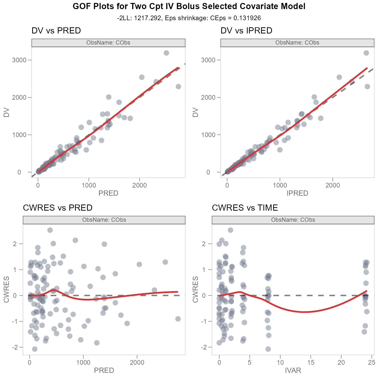
Finally, we’ll use the grid.arrange() function once more, except now we will arrange our title_grob and subtitle_grob with our plot_combined_gof. We will also specify a margin in order to correctly format the spacing for our title_grob and substitle_grob grob() objects, using the heights argument.

# Define margin
margin <- unit(0.5, "line")

# Update combined GOF plot with title and subtitle
updated_plot_combined_gof <-  grid.arrange(title_grob, 
                                           subtitle_grob, 
                                           plot_combined_gof,
                                           heights = unit.c(grobHeight(title_grob) + 2.5*margin, 
                                                            grobHeight(subtitle_grob) + 2.5*margin,
                                                            unit(1,"null")))

The same combined plots figure, but with an overall title added.