Covariate Effects Forest Plots with coveffectsplot

RsNLME package logo

Overview

Forest plots of covariate effects on exposure are a standard way to communicate the clinical relevance of a population PK covariate model. The coveffectsplot package draws these plots from a small summary table with one row per covariate scenario:

Column	Meaning
`paramname`	Exposure metric (e.g. `AUC`, `Cmax`, `Cmin`)
`covname`	Covariate being varied (used for the row facets)
`label`	Scenario within the covariate (e.g. `"15"`, `"Extensive"`)
`mid`	Median ratio of the metric relative to the reference subject
`lower`, `upper`	Uncertainty interval of that ratio
`LABEL`	Text shown in the side table

This vignette shows how to get from an RsNLME fit to that table in six steps, using only package functions and a PML string held in memory:

Fit the covariate model with fitmodel().
Push the final estimates back into the PML with acceptAllEffects().
Add parameter uncertainty by appending a vcvfixef() statement built from fit$thetaCovariance.
Build a small one-at-a-time covariate scenario dataset.
Simulate the scenarios at steady state with simmodel(), once with parameter uncertainty (for the forest) and once with between-subject variability (for the BSV reference band).
Summarise exposure ratios with dplyr and plot with coveffectsplot::forest_plot().

The uncertainty on the forest is uncertainty in the fixed effects only. Between-subject variability (BSV) is displayed as a separate reference band, following Marier, Teuscher, and Mouksassi (2022).

library(Certara.RsNLME)
library(dplyr)
library(tidyr)
library(ggplot2)
library(coveffectsplot)

The NLME engine must be installed and licensed, see the Installation vignette. Model runs in this vignette are written to tempdir().

Data

The example dataset contains 50 subjects dosed 100 mg once daily for 6 days, with rich sampling after the first and last doses and troughs in between. Covariates are body weight (Weight, kg), estimated glomerular filtration rate (eGFR, mL/min), CYP2D6 phenotype (EM, 1 = extensive metabolizer, 0 = poor metabolizer) and population (PAT, 1 = patient, 0 = healthy volunteer).

data_url <- "C:/Users/jcraig/Downloads/RsNLME_CovEffectsPlot/poppkcov.csv"

pk <- read.csv(data_url)
pk$dose_Aa[is.na(pk$dose_Aa)] <- 0
pk$MDV <- as.integer(pk$time == 0) # pre-dose record at time 0 is not an observation

head(pk)
#>    UID time TAD dose_Aa         C      CObs EM PAT   Weight     eGFR MDV
#> 1 1001  0.0 0.0     100 0.0000000 0.0000000  0   1 64.32617 120.8928   1
#> 2 1001  0.5 0.5       0 0.2397747 0.2360399  0   1 64.32617 120.8928   0
#> 3 1001  1.0 1.0       0 0.4492913 0.5040246  0   1 64.32617 120.8928   0
#> 4 1001  2.0 2.0       0 0.7896886 0.9036504  0   1 64.32617 120.8928   0
#> 5 1001  3.0 3.0       0 1.0426083 1.5082850  0   1 64.32617 120.8928   0
#> 6 1001  4.0 4.0       0 1.2254821 1.2184935  0   1 64.32617 120.8928   0

pk %>%
  filter(MDV == 0) %>%
  mutate(
    EM = factor(EM, 0:1, c("Poor metabolizer", "Extensive metabolizer")),
    PAT = factor(PAT, 0:1, c("Healthy", "Patient"))
  ) %>%
  ggplot(aes(time / 24, CObs, group = UID, color = PAT)) +
  geom_line(alpha = 0.5) +
  geom_point(alpha = 0.5, size = 1) +
  scale_y_log10() +
  facet_wrap(~EM) +
  labs(x = "Time (days)", y = "Concentration (mg/L)", color = NULL) +
  theme_bw()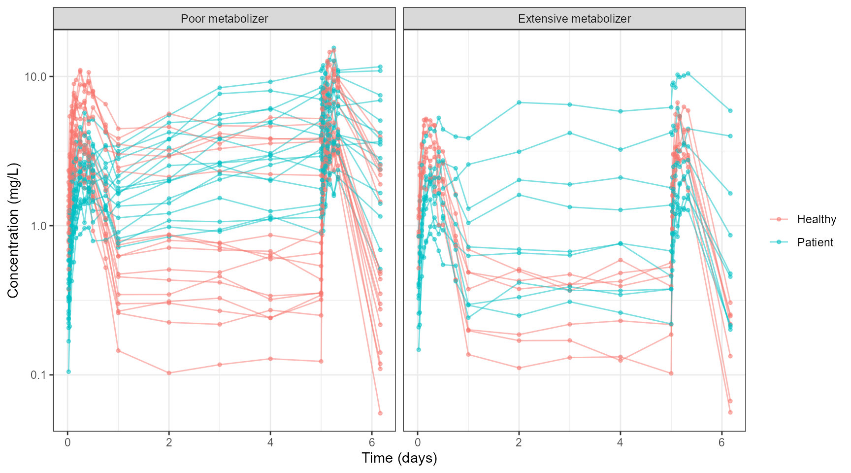

Step 1: Fit the covariate model

The model is a one-compartment model with first-order absorption. Body weight enters allometrically with fixed exponents, eGFR is a power function on clearance, and the two categorical covariates are exponential effects. The centering values in the stparm() statements (70 kg and 90 mL/min) define the reference subject used throughout: 70 kg, eGFR 90 mL/min, poor metabolizer, healthy volunteer.

The PML is a plain character string passed to textualmodel() through the pml argument.

pml_fit <- "
test(){
    cfMicro(A1, Cl / V, first = (Aa = Ka))
    dosepoint(Aa)
    C = A1 / V
    error(CEps = 0.1)
    observe(CObs = C * (1 + CEps))

    stparm(Ka = tvKa)
    stparm(V  = tvV  * (Weight/70)^1    * exp(dVdPAT * (PAT == 1)) * exp(nV))
    stparm(Cl = tvCl * (Weight/70)^0.75 * (eGFR/90)^dCldeGFR *
                exp(dCldEM * (EM == 1)) * exp(dCldPAT * (PAT == 1)) * exp(nCl))

    fcovariate(Weight)
    fcovariate(eGFR)
    fcovariate(EM())
    fcovariate(PAT())

    fixef(tvKa = c(, 0.5, ))
    fixef(tvV  = c(, 10, ))
    fixef(tvCl = c(, 2, ))
    fixef(dCldeGFR = c(, 0.5, ))
    fixef(dVdPAT = c(, 0, ))
    fixef(dCldEM = c(, 0, ))
    fixef(dCldPAT = c(, 0, ))

    ranef(block(nV, nCl) = c(0.1, 0.01, 0.1))
}
"

Map the data columns to the model variables and fit with FOCE ELS.

model <- textualmodel(
  modelName = "PKCov",
  workingDir = file.path(tempdir(), "PKCov"),
  data = pk,
  pml = pml_fit
) %>%
  colMapping(c(
    id = "UID", time = "time", Aa = "dose_Aa", CObs = "CObs",
    Weight = "Weight", eGFR = "eGFR", EM = "EM", PAT = "PAT"
  )) %>%
  addMDV(MDV = "MDV")

fit <- fitmodel(model, params = engineParams(model, method = "FOCE-ELS"))

knitr::kable(fit$Overall[, c("RetCode", "-2LL", "nParm", "nObs", "nSub", "Condition")], digits = 2)

RetCode	-2LL	nParm	nObs	nSub	Condition
2	721.46	11	1150	50	192.26

knitr::kable(fit$theta[, c("Parameter", "Estimate", "Stderr", "CV%")], digits = 3)

Parameter	Estimate	Stderr	CV%
tvKa	0.203	0.008	3.946
tvV	9.401	0.784	8.344
tvCl	1.838	0.116	6.294
dCldeGFR	0.927	0.034	3.690
dVdPAT	1.229	0.102	8.336
dCldEM	0.696	0.047	6.728
dCldPAT	-0.146	0.081	-55.241
CEps	0.150	0.003	1.920

Step 2: Carry the final estimates into the PML

acceptAllEffects() reads the results in the model’s working directory and rewrites the fixef(), ranef() and error() statements with the final estimates. The updated PML lives in model@statements; collapse it to a single string so it can be edited and reused.

model_final <- acceptAllEffects(model)
pml_final <- paste(unlist(model_final@statements), collapse = "\n")
cat(pml_final)
#> test(){
#>     cfMicro(A1, Cl / V, first = (Aa = Ka))
#>     dosepoint(Aa)
#>     C = A1 / V
#>     error(CEps = 0.149701771240153)
#>     observe(CObs = C * (1 + CEps))
#> 
#>     stparm(Ka = tvKa)
#>     stparm(V  = tvV  * (Weight/70)^1    * exp(dVdPAT * (PAT == 1)) * exp(nV))
#>     stparm(Cl = tvCl * (Weight/70)^0.75 * (eGFR/90)^dCldeGFR *
#>                 exp(dCldEM * (EM == 1)) * exp(dCldPAT * (PAT == 1)) * exp(nCl))
#> 
#>     fcovariate(Weight)
#>     fcovariate(eGFR)
#>     fcovariate(EM())
#>     fcovariate(PAT())
#> 
#>     fixef(tvKa = c(, 0.203446083595785, ))
#>     fixef(tvV = c(, 9.40066213082382, ))
#>     fixef(tvCl = c(, 1.83750082810562, ))
#>     fixef(dCldeGFR = c(, 0.926881932316507, ))
#>     fixef(dVdPAT = c(, 1.22890700341193, ))
#>     fixef(dCldEM = c(, 0.695689705521502, ))
#>     fixef(dCldPAT = c(, -0.146227039637686, ))
#> 
#>     ranef(block(nV, nCl) = c(0.13171206, 0.088404018, 0.07994101))
#> }

Step 3: Add parameter uncertainty with `vcvfixef()`

The PML statement vcvfixef() tells the engine to draw a new fixed-effect vector from a multivariate normal distribution for every simulation replicate. It takes the variance-covariance matrix of the fixed effects as its lower triangle, written row by row: Var(theta1), Cov(theta2, theta1), Var(theta2), Cov(theta3, theta1), ....

fit$thetaCovariance holds exactly this matrix (lower triangle, with a Scenario label column in front). The residual error parameter CEps is part of it but is not needed for simulating concentrations without residual error, so it is dropped.

theta_cov <- as.matrix(fit$thetaCovariance[, -1]) # drop the Scenario column
dimnames(theta_cov) <- list(colnames(theta_cov), colnames(theta_cov))
theta_cov[upper.tri(theta_cov)] <- t(theta_cov)[upper.tri(theta_cov)] # mirror to a full matrix

thetas <- setdiff(colnames(theta_cov), "CEps")
theta_cov <- theta_cov[thetas, thetas]
knitr::kable(theta_cov, digits = 5)

	tvKa	tvV	tvCl	dCldeGFR	dVdPAT	dCldEM	dCldPAT
tvKa	0.00006	0.00302	0.00012	0.00008	0.00000	-0.00004	-0.00004
tvV	0.00302	0.61522	0.06923	0.00157	-0.05033	0.00057	-0.03846
tvCl	0.00012	0.06923	0.01337	0.00099	-0.00722	-0.00112	-0.00683
dCldeGFR	0.00008	0.00157	0.00099	0.00117	-0.00036	-0.00040	-0.00034
dVdPAT	0.00000	-0.05033	-0.00722	-0.00036	0.01050	-0.00035	0.00714
dCldEM	-0.00004	0.00057	-0.00112	-0.00040	-0.00035	0.00219	-0.00035
dCldPAT	-0.00004	-0.03846	-0.00683	-0.00034	0.00714	-0.00035	0.00652


# Row-wise lower triangle of theta_cov, in the order vcvfixef() expects
vcv_values <- t(theta_cov)[upper.tri(theta_cov, diag = TRUE)]

vcvfixef_line <- sprintf(
  "    vcvfixef(block(%s) = c(%s))",
  paste(thetas, collapse = ", "),
  paste(signif(vcv_values, 8), collapse = ", ")
)

Two edits on the PML string produce the uncertainty simulation model: set the random effects to (effectively) zero so that only parameter uncertainty is simulated, and insert the vcvfixef() line before the closing brace.

pml_unc <- sub("ranef\\([^\n]*", "ranef(block(nV, nCl) = c(1e-12, 0, 1e-12))", pml_final)
pml_unc <- sub("\\}\\s*$", paste0(vcvfixef_line, "\n}"), pml_unc)
cat(pml_unc)
#> test(){
#>     cfMicro(A1, Cl / V, first = (Aa = Ka))
#>     dosepoint(Aa)
#>     C = A1 / V
#>     error(CEps = 0.149701771240153)
#>     observe(CObs = C * (1 + CEps))
#> 
#>     stparm(Ka = tvKa)
#>     stparm(V  = tvV  * (Weight/70)^1    * exp(dVdPAT * (PAT == 1)) * exp(nV))
#>     stparm(Cl = tvCl * (Weight/70)^0.75 * (eGFR/90)^dCldeGFR *
#>                 exp(dCldEM * (EM == 1)) * exp(dCldPAT * (PAT == 1)) * exp(nCl))
#> 
#>     fcovariate(Weight)
#>     fcovariate(eGFR)
#>     fcovariate(EM())
#>     fcovariate(PAT())
#> 
#>     fixef(tvKa = c(, 0.203446083595785, ))
#>     fixef(tvV = c(, 9.40066213082382, ))
#>     fixef(tvCl = c(, 1.83750082810562, ))
#>     fixef(dCldeGFR = c(, 0.926881932316507, ))
#>     fixef(dVdPAT = c(, 1.22890700341193, ))
#>     fixef(dCldEM = c(, 0.695689705521502, ))
#>     fixef(dCldPAT = c(, -0.146227039637686, ))
#> 
#>     ranef(block(nV, nCl) = c(1e-12, 0, 1e-12))
#>     vcvfixef(block(tvKa, tvV, tvCl, dCldeGFR, dVdPAT, dCldEM, dCldPAT) = c(6.4448829e-05, 0.0030173853, 0.61522026, 0.00011757541, 0.069226099, 0.013374252, 8.3110331e-05, 0.0015705288, 0.00099075908, 0.0011700714, 2.1045616e-06, -0.050334733, -0.007220356, -0.00035654749, 0.010495316, -3.7423564e-05, 0.00057271665, -0.0011170658, -0.00040121229, -0.00034913771, 0.0021909248, -3.6161251e-05, -0.03846472, -0.0068253611, -0.00033813768, 0.0071353497, -0.00034923941, 0.0065249618))
#> }

Step 4: Covariate scenarios

Each scenario is one virtual subject receiving 100 mg once daily at steady state (SS = 1, II = 24). Starting from the reference subject, one covariate at a time is set to a clinically relevant value: eGFR at the renal impairment cut-offs, body weight across the range seen in the study, and the two categorical covariates switched to their non-reference level. The covname and label columns are carried along so they can be joined back to the simulation output later.

reference <- data.frame(Weight = 70, eGFR = 90, EM = 0, PAT = 0)

scenarios <- bind_rows(
  reference %>% mutate(covname = "Reference", label = "70 kg / eGFR 90 / PM / Healthy"),
  reference %>% select(-eGFR) %>% crossing(eGFR = c(15, 30, 60, 125)) %>%
    mutate(covname = "eGFR", label = as.character(eGFR)),
  reference %>% select(-Weight) %>% crossing(Weight = c(40, 55, 63, 77, 83, 88)) %>%
    mutate(covname = "Weight", label = as.character(Weight)),
  reference %>% mutate(EM = 1, covname = "EM", label = "Extensive"),
  reference %>% mutate(PAT = 1, covname = "PAT", label = "Patients")
) %>%
  mutate(ID = row_number(), time = 0, dose_Aa = 100, SS = 1, II = 24, .before = 1)

knitr::kable(scenarios)

ID	dose_Aa	SS	II	Weight	eGFR	EM	PAT	covname	label
1	100	1	24	70	90	0	0	Reference	70 kg / eGFR 90 / PM / Healthy
2	100	1	24	70	15	0	0	eGFR	15
3	100	1	24	70	30	0	0	eGFR	30
4	100	1	24	70	60	0	0	eGFR	60
5	100	1	24	70	125	0	0	eGFR	125
6	100	1	24	40	90	0	0	Weight	40
7	100	1	24	55	90	0	0	Weight	55
8	100	1	24	63	90	0	0	Weight	63
9	100	1	24	77	90	0	0	Weight	77
10	100	1	24	83	90	0	0	Weight	83
11	100	1	24	88	90	0	0	Weight	88
12	100	1	24	70	90	1	0	EM	Extensive
13	100	1	24	70	90	0	1	PAT	Patients

Step 5: Simulate at steady state

Both simulations request the same table: concentration C and clearance Cl over one dosing interval. addSteadyState() maps the SS and II columns.

sim_table <- tableParams(
  name = "SimTable.csv",
  timesList = seq(0, 24, by = 0.25),
  variablesList = c("C", "Cl"),
  forSimulation = TRUE
)

The uncertainty simulation runs all scenarios with the vcvfixef() model. Each of the 200 replicates uses a different draw of the fixed effects, and within a replicate every scenario shares that draw, which is what allows ratios to the reference subject to be formed replicate by replicate.

model_unc <- textualmodel(
  modelName = "PKCovUncertainty",
  workingDir = file.path(tempdir(), "PKCovUncertainty"),
  data = scenarios,
  pml = pml_unc
) %>%
  colMapping(c(
    id = "ID", time = "time", Aa = "dose_Aa",
    Weight = "Weight", eGFR = "eGFR", EM = "EM", PAT = "PAT"
  )) %>%
  addSteadyState(SS = "SS", II = "II")

sim_unc <- simmodel(
  model_unc,
  NlmeSimulationParams(numReplicates = 200, seed = 1234, simulationTables = sim_table)
)

The BSV simulation uses the fitted model unchanged (random effects on, no vcvfixef()) and only the reference subject, replicated 1000 times.

model_bsv <- textualmodel(
  modelName = "PKCovBSV",
  workingDir = file.path(tempdir(), "PKCovBSV"),
  data = filter(scenarios, covname == "Reference"),
  pml = pml_final
) %>%
  colMapping(c(
    id = "ID", time = "time", Aa = "dose_Aa",
    Weight = "Weight", eGFR = "eGFR", EM = "EM", PAT = "PAT"
  )) %>%
  addSteadyState(SS = "SS", II = "II")

sim_bsv <- simmodel(
  model_bsv,
  NlmeSimulationParams(numReplicates = 1000, seed = 5678, simulationTables = sim_table)
)

Simulation tables are returned in memory, named after the tableParams() name. The replicate is in # repl and the subject in id5.

head(sim_unc$SimTable)
#>    # repl    id1    id2    id3    id4   id5  time         C       Cl
#>     <int> <lgcl> <lgcl> <lgcl> <lgcl> <int> <num>     <num>    <num>
#> 1:      0     NA     NA     NA     NA     1  0.00 0.4749591 1.787299
#> 2:      0     NA     NA     NA     NA     1  0.25 0.9698019 1.787299
#> 3:      0     NA     NA     NA     NA     1  0.50 1.4161502 1.787299
#> 4:      0     NA     NA     NA     NA     1  0.75 1.8175154 1.787299
#> 5:      0     NA     NA     NA     NA     1  1.00 2.1771838 1.787299
#> 6:      0     NA     NA     NA     NA     1  1.25 2.4982300 1.787299

A quick look at the simulated profiles shows the effect of each scenario and the width of the parameter-uncertainty band.

sim_unc$SimTable %>%
  rename(Replicate = `# repl`, ID = id5) %>%
  left_join(select(scenarios, ID, covname, label), by = "ID") %>%
  group_by(ID, covname, label, time) %>%
  summarise(
    median = median(C),
    lower = quantile(C, 0.05),
    upper = quantile(C, 0.95),
    .groups = "drop"
  ) %>%
  ggplot(aes(time, median)) +
  geom_ribbon(aes(ymin = lower, ymax = upper), fill = "steelblue", alpha = 0.3) +
  geom_line() +
  facet_wrap(~ reorder(ifelse(covname == "Reference", label, paste(covname, label)), ID), ncol = 4) +
  labs(x = "Time after dose (h)", y = "Concentration (mg/L)") +
  theme_bw()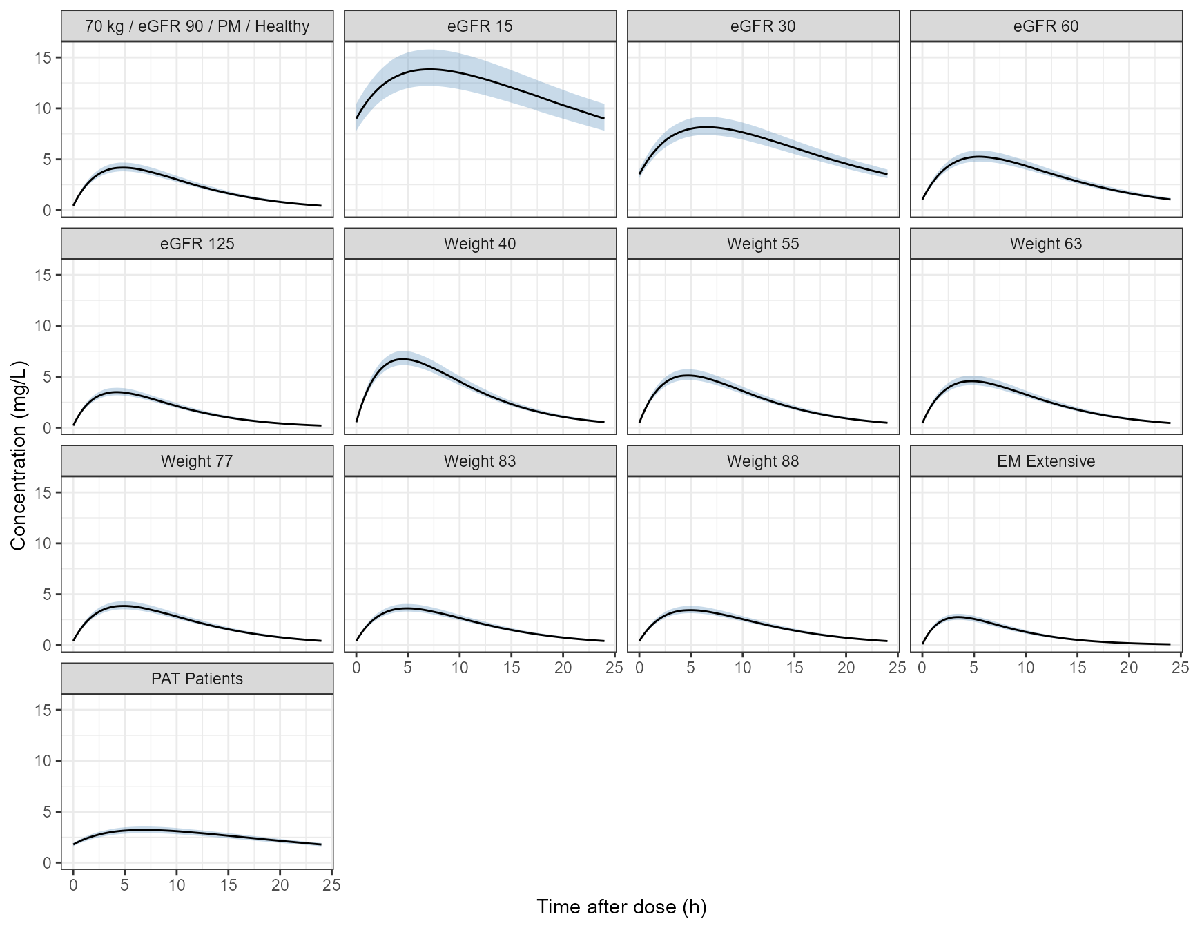

Step 6: Exposure metrics and the forest table

Three steady-state exposure metrics are derived per replicate and subject: AUC over the dosing interval (Dose / Cl), Cmax and the trough Cmin. Stacking both simulations first means the metrics are computed once.

dose <- 100

metrics <- bind_rows(uncertainty = sim_unc$SimTable, bsv = sim_bsv$SimTable, .id = "source") %>%
  rename(Replicate = `# repl`, ID = id5) %>%
  group_by(source, Replicate, ID) %>%
  summarise(
    AUC = dose / first(Cl),
    Cmax = max(C),
    Cmin = C[time == 24],
    .groups = "drop"
  ) %>%
  pivot_longer(c(AUC, Cmax, Cmin), names_to = "paramname", values_to = "value") %>%
  left_join(select(scenarios, ID, covname, label), by = "ID")

head(metrics)
#> # A tibble: 6 × 7
#>   source Replicate    ID paramname  value covname   label                       
#>   <chr>      <int> <int> <chr>      <dbl> <chr>     <chr>                       
#> 1 bsv            0     1 AUC       52.2   Reference 70 kg / eGFR 90 / PM / Heal…
#> 2 bsv            0     1 Cmax       4.22  Reference 70 kg / eGFR 90 / PM / Heal…
#> 3 bsv            0     1 Cmin       0.353 Reference 70 kg / eGFR 90 / PM / Heal…
#> 4 bsv            1     1 AUC       58.6   Reference 70 kg / eGFR 90 / PM / Heal…
#> 5 bsv            1     1 Cmax       4.14  Reference 70 kg / eGFR 90 / PM / Heal…
#> 6 bsv            1     1 Cmin       0.646 Reference 70 kg / eGFR 90 / PM / Heal…

For the covariate rows, each scenario is divided by the reference subject within the same replicate, then the ratios are summarised across replicates by their median and 90% interval.

forest_cov <- metrics %>%
  filter(source == "uncertainty") %>%
  group_by(Replicate, paramname) %>%
  mutate(ratio = value / value[covname == "Reference"]) %>%
  filter(covname != "Reference") %>%
  group_by(paramname, covname, label) %>%
  summarise(
    mid = median(ratio),
    lower = quantile(ratio, 0.05, names = FALSE),
    upper = quantile(ratio, 0.95, names = FALSE),
    .groups = "drop"
  )

For the BSV rows, each simulated reference subject is divided by the median reference subject. The 25th-75th and 5th-95th percentiles show where 50% and 90% of subjects fall, giving the reader a scale for the covariate effects.

forest_bsv <- metrics %>%
  filter(source == "bsv") %>%
  group_by(paramname) %>%
  mutate(ratio = value / median(value)) %>%
  reframe(
    covname = "BSV",
    label = c("90% of subjects", "50% of subjects"),
    mid = 1,
    lower = quantile(ratio, c(0.05, 0.25), names = FALSE),
    upper = quantile(ratio, c(0.95, 0.75), names = FALSE)
  )

Combine, add the table text, and order the factor levels: covname levels set the facet order from top to bottom, and label levels are drawn from bottom to top within a facet.

forest_data <- bind_rows(forest_cov, forest_bsv) %>%
  mutate(
    LABEL = sprintf("%.2f [%.2f, %.2f]", mid, lower, upper),
    paramname = factor(paramname, levels = c("AUC", "Cmax", "Cmin")),
    covname = factor(covname, levels = c("eGFR", "Weight", "EM", "PAT", "BSV")),
    label = factor(label, levels = c(
      "15", "30", "60", "125",
      "40", "55", "63", "77", "83", "88",
      "Extensive", "Patients",
      "90% of subjects", "50% of subjects"
    ))
  )

knitr::kable(filter(forest_data, paramname == "AUC"), digits = 2)

paramname	covname	label	mid	lower	upper	LABEL
AUC	EM	Extensive	0.50	0.47	0.54	0.50 [0.47, 0.54]
AUC	PAT	Patients	1.17	1.02	1.32	1.17 [1.02, 1.32]
AUC	Weight	40	1.52	1.52	1.52	1.52 [1.52, 1.52]
AUC	Weight	55	1.20	1.20	1.20	1.20 [1.20, 1.20]
AUC	Weight	63	1.08	1.08	1.08	1.08 [1.08, 1.08]
AUC	Weight	77	0.93	0.93	0.93	0.93 [0.93, 0.93]
AUC	Weight	83	0.88	0.88	0.88	0.88 [0.88, 0.88]
AUC	Weight	88	0.84	0.84	0.84	0.84 [0.84, 0.84]
AUC	eGFR	125	0.74	0.72	0.75	0.74 [0.72, 0.75]
AUC	eGFR	15	5.28	4.79	5.82	5.28 [4.79, 5.82]
AUC	eGFR	30	2.78	2.61	2.94	2.78 [2.61, 2.94]
AUC	eGFR	60	1.46	1.43	1.49	1.46 [1.43, 1.49]
AUC	BSV	90% of subjects	1.00	0.65	1.60	1.00 [0.65, 1.60]
AUC	BSV	50% of subjects	1.00	0.83	1.21	1.00 [0.83, 1.21]

Forest plots

forest_plot() draws the plot and, with table_position = "right", the side table. The gray band marks the 0.8-1.25 no-effect region, the blue points and lines are the medians and 90% intervals from parameter uncertainty, and the red BSV rows give the spread between subjects at the reference covariates.

covname_labels <- c(
  eGFR = "eGFR\n(mL/min)", Weight = "Weight\n(kg)", EM = "CYP2D6\nmetabolizer",
  PAT = "Population", BSV = "Between-subject\nvariability"
)

forest_auc <- forest_plot(
  filter(forest_data, paramname == "AUC"),
  ref_area = c(0.8, 1.25),
  x_range = c(0.4, 6),
  xlabel = "Fold change in AUC relative to the reference subject",
  facet_formula = "covname ~ .",
  facet_switch = "y",
  facet_scales = "free_y",
  facet_space = "free",
  facet_labeller = labeller(covname = covname_labels),
  strip_placement = "outside",
  ref_legend_text = "Reference (vertical line)\nClinically relevant limits 0.8-1.25 (gray area)",
  area_legend_text = "Reference (vertical line)\nClinically relevant limits 0.8-1.25 (gray area)",
  interval_legend_text = "Median (points)\n90% CI (horizontal lines)",
  interval_bsv_text = "BSV (points)\nPrediction intervals (horizontal lines)",
  combine_area_ref_legend = TRUE,
  legend_order = c("pointinterval", "ref", "area"),
  legend_position = "top",
  logxscale = TRUE,
  major_x_ticks = c(0.5, 0.8, 1, 1.25, 2, 4),
  major_x_labels = c("1/2", "0.8", "1", "1.25", "2", "4"),
  table_position = "right",
  table_text_size = 4,
  plot_table_ratio = 3,
  show_table_facet_strip = "none",
  base_size = 14,
  plot_title = ""
)

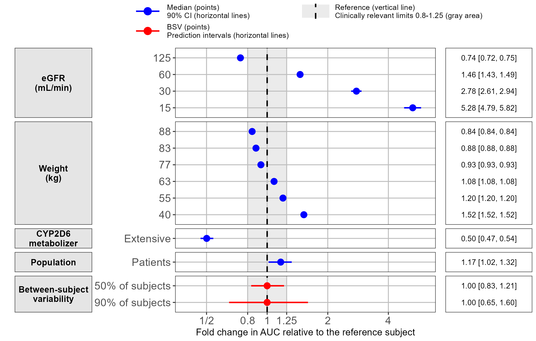
Note that the body weight rows have no visible interval. The allometric exponents were fixed rather than estimated, so the weight effect carries no parameter uncertainty; only estimated fixed effects contribute to the interval.

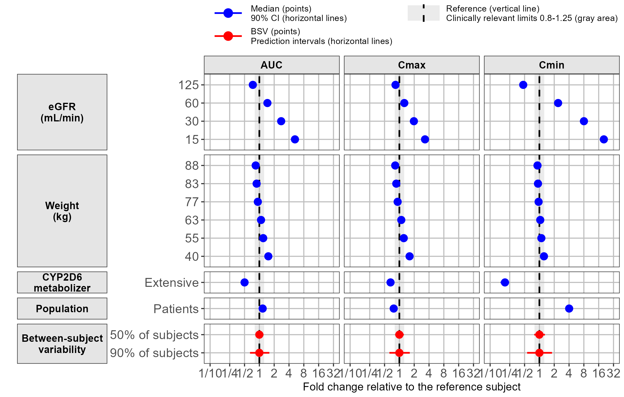
Adding paramname to the facet formula shows all three metrics side by side.

forest_plot(
  forest_data,
  ref_area = c(0.8, 1.25),
  x_range = c(0.1, 32),
  xlabel = "Fold change relative to the reference subject",
  facet_formula = "covname ~ paramname",
  facet_switch = "y",
  facet_scales = "free_y",
  facet_space = "free",
  facet_labeller = labeller(covname = covname_labels),
  strip_placement = "outside",
  ref_legend_text = "Reference (vertical line)\nClinically relevant limits 0.8-1.25 (gray area)",
  area_legend_text = "Reference (vertical line)\nClinically relevant limits 0.8-1.25 (gray area)",
  interval_legend_text = "Median (points)\n90% CI (horizontal lines)",
  interval_bsv_text = "BSV (points)\nPrediction intervals (horizontal lines)",
  combine_area_ref_legend = TRUE,
  legend_order = c("pointinterval", "ref", "area"),
  legend_position = "top",
  logxscale = TRUE,
  major_x_ticks = c(0.1, 0.25, 0.5, 1, 2, 4, 8, 16, 32),
  major_x_labels = c("1/10", "1/4", "1/2", "1", "2", "4", "8", "16", "32"),
  table_position = "none",
  base_size = 14,
  plot_title = ""
)

Summary

The whole workflow uses two PML strings and two simmodel() calls:

fitmodel() estimates the covariate model; acceptAllEffects() writes the estimates back into the PML.
fit$thetaCovariance becomes a vcvfixef() statement, appended to the PML with sub(), so that simmodel(numReplicates = n) samples the fixed effects n times.
The covariate scenarios are ordinary rows in the simulation dataset; the reference subject is just another row, which makes within-replicate ratios a one-line dplyr operation.
coveffectsplot::forest_plot() consumes the summarised ratios directly.

A nonparametric alternative to vcvfixef() is to run bootstrap() and simulate each successful bootstrap replicate’s fixed effects instead; the downstream steps are unchanged.

References

Marier JF, Teuscher N, Mouksassi MS. Evaluation of covariate effects using forest plots and introduction to the coveffectsplot R package. CPT Pharmacometrics Syst Pharmacol. 2022;11(10):1283-1293. doi:10.1002/psp4.12829
U.S. Food and Drug Administration. Population Pharmacokinetics. Guidance for Industry. February 2022. https://www.fda.gov/media/128793/download
Certara. Phoenix PML: Simulation with parameter uncertainty included.