Generating vachette inputs from RsNLME

This vignette shows how to generate the three datasets that vachette::vachette_data() requires (obs.data, typ.data, sim.data) directly from a fitted Certara.RsNLME model. It focuses on the trickiest piece: building typ.data, the typical-curve table that contains one trajectory per unique covariate combination present in the observed data.

The model setup mirrors the conventions in the RsNLME Covariate Models vignette; the simulation mechanics (tableParams(), simmodel(), NlmeSimulationParams()) follow the Simulation in RsNLME vignette.

library(vachette)

library(Certara.RsNLME)
library(dplyr)
library(tidyr)
library(tidyvpc)
library(ggplot2)

What vachette needs

vachette_data() accepts three data frames (see ?vachette_data for the full column reference):

Dataset	Required columns	Source in this vignette
`obs.data`	`ID`, `x` (time), `OBS` (DV), `dosenr`, plus covariate columns	`pkData` (renamed)
`sim.data`	`ID`, `x`, `OBS`, `REP`, `dosenr`, plus covariate columns	`simmodel()` with replicates
`typ.data`	`ID`, `x`, `PRED`, `dosenr`, plus covariate columns	`simmodel()` with frozen IIV + synthetic input dataset

dosenr identifies a dose interval (single-dose data here, so all rows get dosenr = 1). REP is the replicate index in sim.data.

1. Build and fit the covariate model

We use the built-in pkData (16 subjects, 2-cpt IV bolus). Following the SCM-best result from the RsNLME covariate-model vignette, we add BodyWeight as a continuous covariate on V/Cl and additionally include Gender as a categorical covariate on Cl to demonstrate both covariate types.

workingDir <- file.path(tempdir(), "rsnlme_vachette")
dir.create(workingDir, recursive = TRUE, showWarnings = FALSE)

baseModel <- pkmodel(
  numCompartments = 2,
  data = pkData,
  ID = "Subject", Time = "Act_Time",
  A1 = "Amount", CObs = "Conc",
  modelName = "rsnlme_vachette_base",
  workingDir = workingDir
) %>%
  addCovariate(
    covariate = "BodyWeight",
    type = "Continuous",
    effect = c("V", "Cl"),
    direction = "Forward",
    center = "Median"
  ) %>%
  addCovariate(
    covariate = "Gender",
    type = "Categorical",
    effect = "Cl",
    levels = c(0, 1),
    labels = c("male", "female")
  )

fitJob <- fitmodel(baseModel)

fitJob$Overall
#>    Scenario RetCode    LogLik     -2LL      AIC      BIC nParm  nObs  nSub
#>      <char>   <int>     <num>    <num>    <num>    <num> <int> <int> <int>
#> 1: WorkFlow       1 -607.4505 1214.901 1238.901 1271.523    12   112    16
#>    EpsShrinkage Condition
#>           <num>    <lgcl>
#> 1:      0.12993        NA

2. Build `obs.data` from `pkData`

pkData already contains everything we need; only column renaming and a dosenr flag are required.

obs <- pkData %>%
  rename(ID = Subject, x = Act_Time, OBS = Conc) %>%
  mutate(dosenr = 1L) %>%
  select(ID, x, OBS, dosenr, BodyWeight, Gender, Age)

head(obs)
#>       ID     x   OBS dosenr BodyWeight Gender   Age
#>    <num> <num> <num>  <int>      <num> <char> <num>
#> 1:     1  0.00  2010      1         73   male    22
#> 2:     1  0.26  1330      1         73   male    22
#> 3:     1  1.10   565      1         73   male    22
#> 4:     1  2.10   216      1         73   male    22
#> 5:     1  4.13   180      1         73   male    22
#> 6:     1  8.17   120      1         73   male    22

3. Generate `sim.data` via `simmodel()` with a custom output table

For the simulated VPC dataset, we use simmodel() rather than vpcmodel() so we can control exactly which columns appear in the output. Putting the covariate names into variablesList echoes them into the output table next to the simulated CObs. keepSource = TRUE matches the simulated time grid to the observed grid, which is what vachette expects when comparing observed and simulated trajectories.

simModel <- copyModel(
  baseModel,
  acceptAllEffects = TRUE,
  modelName = "rsnlme_vachette_sim"
)

simTable <- tableParams(
  name = "sim_replicates.csv",
  variablesList = c("CObs", "C", "BodyWeight", "Gender"),
  keepSource = TRUE,
  forSimulation = TRUE
)

simParams <- NlmeSimulationParams(
  numReplicates = 50,
  seed = 1,
  simulationTables = simTable
)

simJob <- simmodel(simModel, simParams)

The simulation table is returned in the result list under its file name (without extension). When the simulator writes a categorical covariate to a table it uses the internal numeric code (0 / 1) rather than the labels declared in addCovariate(), and the replicate index is written under a column literally named # repl. We define a small helper to map the numeric codes back to "male" / "female" so the covariate values match between obs and sim:

recode_gender <- function(g) {
  g <- as.character(g)
  dplyr::case_when(
    g %in% c("0", "male")   ~ "male",
    g %in% c("1", "female") ~ "female",
    TRUE ~ g
  )
}

If you defined your categorical levels with a different mapping in addCovariate(), adjust recode_gender() (or write a similar helper) so the simulated and observed factor levels line up.

Now reshape the simulation output into the vachette schema:

sim_raw <- as.data.frame(simJob$sim_replicates)

sim <- sim_raw %>%
  rename(REP = `# repl`, ID = id5, x = time, OBS = CObs) %>%
  mutate(
    dosenr = 1L,
    Gender = recode_gender(Gender)
  ) %>%
  filter(!is.na(OBS)) %>%
  select(REP, ID, x, OBS, dosenr, BodyWeight, Gender)

head(sim)
#>   REP ID    x       OBS dosenr BodyWeight Gender
#> 1   0  1 0.00 1565.0523      1         73   male
#> 2   0  1 0.26 1306.5094      1         73   male
#> 3   0  1 1.10  571.4460      1         73   male
#> 4   0  1 2.10  319.5886      1         73   male
#> 5   0  1 4.13  152.9584      1         73   male
#> 6   0  1 8.17  104.7707      1         73   male

4. Generate `typ.data` (the tricky part)

typ.data is one typical trajectory per unique covariate combination in obs.data. The strategy:

Build a synthetic input dataset: one row per (unique covariate combination × dense time grid), with a dose at t = 0.
copyModel(..., acceptAllEffects = TRUE) to fix the fitted thetas.
randomEffect(..., isFrozen = TRUE, value = ~0) to suppress IIV so the simulated trajectory is the population prediction.
dataMapping() + colMapping() to swap the synthetic input onto the model.
simmodel() with a tableParams() definition that captures the central concentration C plus the covariate columns.

4a. Synthetic input dataset

unique_covs <- pkData %>%
  distinct(BodyWeight, Gender) %>%
  mutate(SyntheticID = 1000000L + row_number())

t_grid <- c(0, seq(0.1, max(pkData$Act_Time, na.rm = TRUE) * 1.1,
                   length.out = 199))

typ_input <- unique_covs %>%
  tidyr::expand_grid(Act_Time = t_grid) %>%
  mutate(
    Subject = SyntheticID,
    Amount  = ifelse(Act_Time == 0, 25000, NA_real_),
    Conc    = NA_real_
  ) %>%
  select(Subject, Act_Time, Amount, Conc, BodyWeight, Gender)

cat("unique covariate combinations:", nrow(unique_covs),
    "  time grid points:", length(t_grid),
    "  synthetic rows:", nrow(typ_input), "\n")
#> unique covariate combinations: 13   time grid points: 200   synthetic rows: 2600

4b–d. Build the typical-curve model

copyModel(acceptAllEffects = TRUE) carries the fitted thetas onto a new (still built-in, not textual) model. We then freeze every random effect at variance 0 so each synthetic ID’s realization is exactly η = 0 and the simulated C is the population prediction (PRED).

typModel <- copyModel(
  baseModel,
  acceptAllEffects = TRUE,
  modelName = "rsnlme_vachette_typ"
) %>%
  randomEffect(
    effect   = c("nV", "nCl", "nV2", "nCl2"),
    value    = rep(0, 4),
    isFrozen = TRUE
  ) %>%
  dataMapping(typ_input) %>%
  colMapping(c(
    id   = "Subject",
    time = "Act_Time",
    A1   = "Amount",
    CObs = "Conc"
  ))

randomEffect() requires a built-in (non-textual) model, so call it before any editModel() step. See ?Certara.RsNLME::randomEffect.

4e. Simulate and reshape

typTable <- tableParams(
  name = "typ_curves.csv",
  timesList = t_grid,
  variablesList = c("C", "BodyWeight", "Gender"),
  forSimulation = TRUE
)

typParams <- NlmeSimulationParams(
  numReplicates = 1,
  seed = 1,
  simulationTables = typTable
)

typJob <- simmodel(typModel, typParams)

typ_raw <- as.data.frame(typJob$typ_curves)

typ <- typ_raw %>%
  rename(ID = id5, x = time, PRED = C) %>%
  mutate(
    dosenr = 1L,
    Gender = recode_gender(Gender)
  ) %>%
  select(ID, x, PRED, dosenr, BodyWeight, Gender)

stopifnot(nrow(typ) == nrow(unique_covs) * length(t_grid))
head(typ)
#>        ID         x      PRED dosenr BodyWeight Gender
#> 1 1000001 0.0000000 1309.9830      1         73   male
#> 2 1000001 0.1000000 1161.3947      1         73   male
#> 3 1000001 0.2340505  992.6181      1         73   male
#> 4 1000001 0.3681010  853.0392      1         73   male
#> 5 1000001 0.5021515  737.5219      1         73   male
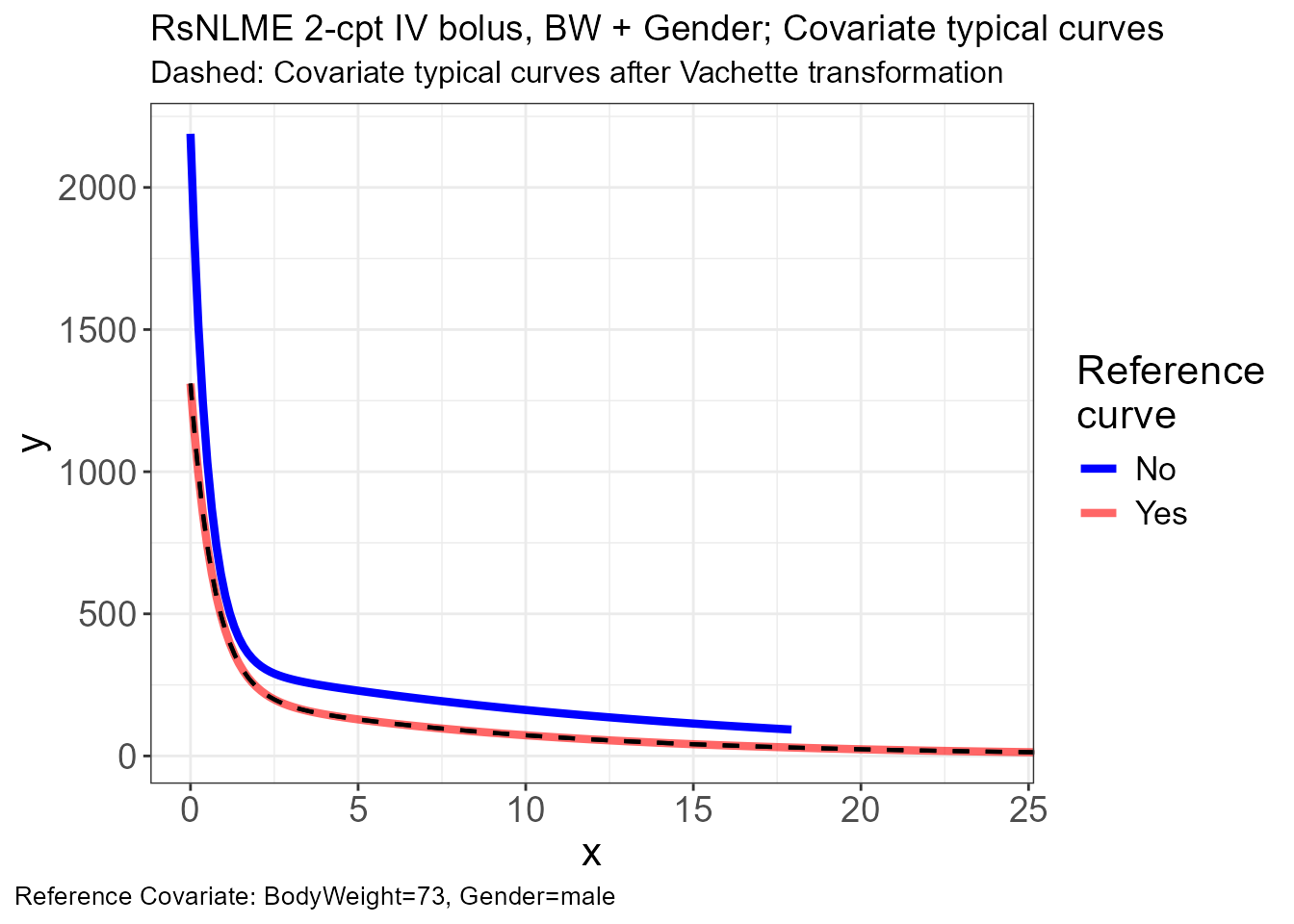
#> 6 1000001 0.6362020  641.8350      1         73   male

5. Run vachette on one reference + one query combination

For a clean demonstration we filter the three datasets to one reference combination and one query combination with semi_join(). This keeps the vachette plot panel readable: one typical reference curve, one typical query curve, and the observations / simulations that belong to those two combinations.

The reference combination must exist in typ.data and obs.data — vachette_data() matches it by exact equality on the named covariate columns. Here we pick (BodyWeight = 73, Gender = "male") as the reference (Subject 1’s covariates) and (BodyWeight = 50, Gender = "female") as the query (Subject 10’s covariates).

ref_combo   <- tibble(BodyWeight = 73, Gender = "male")
query_combo <- tibble(BodyWeight = 50, Gender = "female")
keep_combos <- bind_rows(ref_combo, query_combo)

obs_pair <- obs %>% semi_join(keep_combos, by = c("BodyWeight", "Gender"))
typ_pair <- typ %>% semi_join(keep_combos, by = c("BodyWeight", "Gender"))
sim_pair <- sim %>% semi_join(keep_combos, by = c("BodyWeight", "Gender"))

vd <- vachette_data(
  obs.data   = obs_pair,
  typ.data   = typ_pair,
  sim.data   = sim_pair,
  covariates = c(BodyWeight = ref_combo$BodyWeight,
                 Gender     = ref_combo$Gender),
  model.name = "RsNLME 2-cpt IV bolus, BW + Gender"
) %>%
  apply_transformations()

p.obs.ref.query(vd)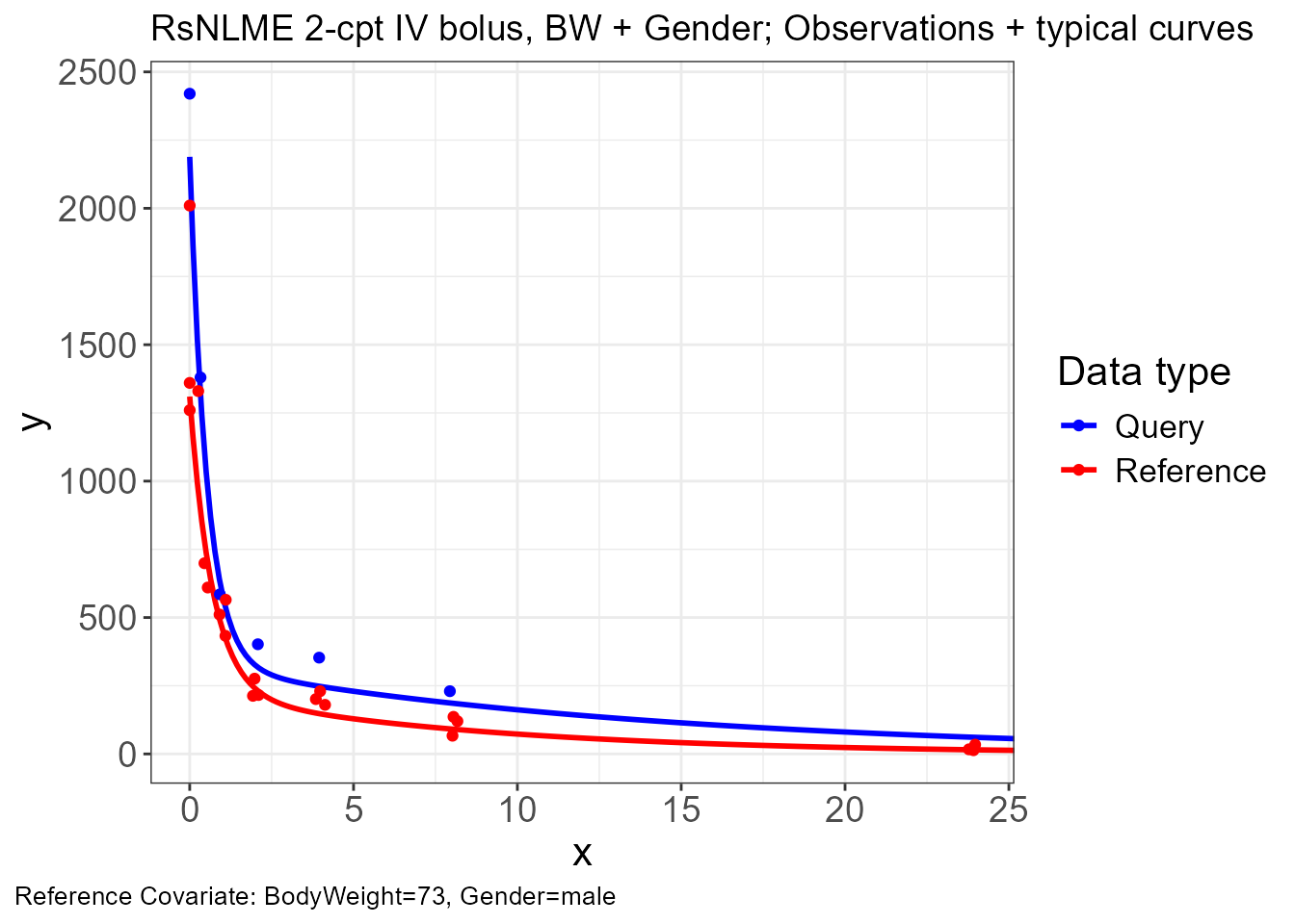

p.vachette(vd)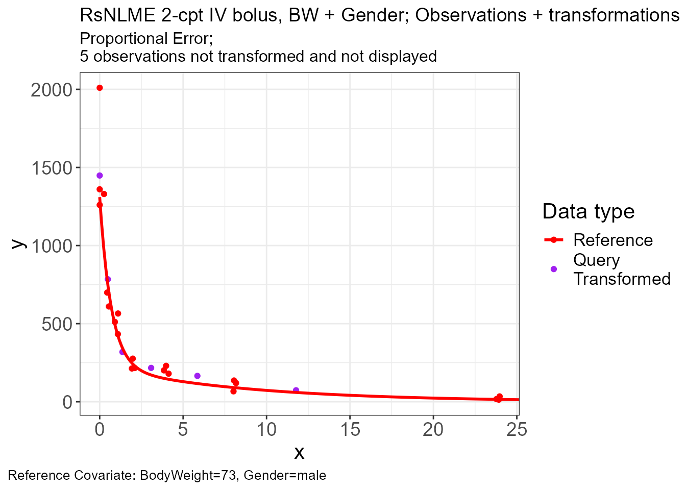

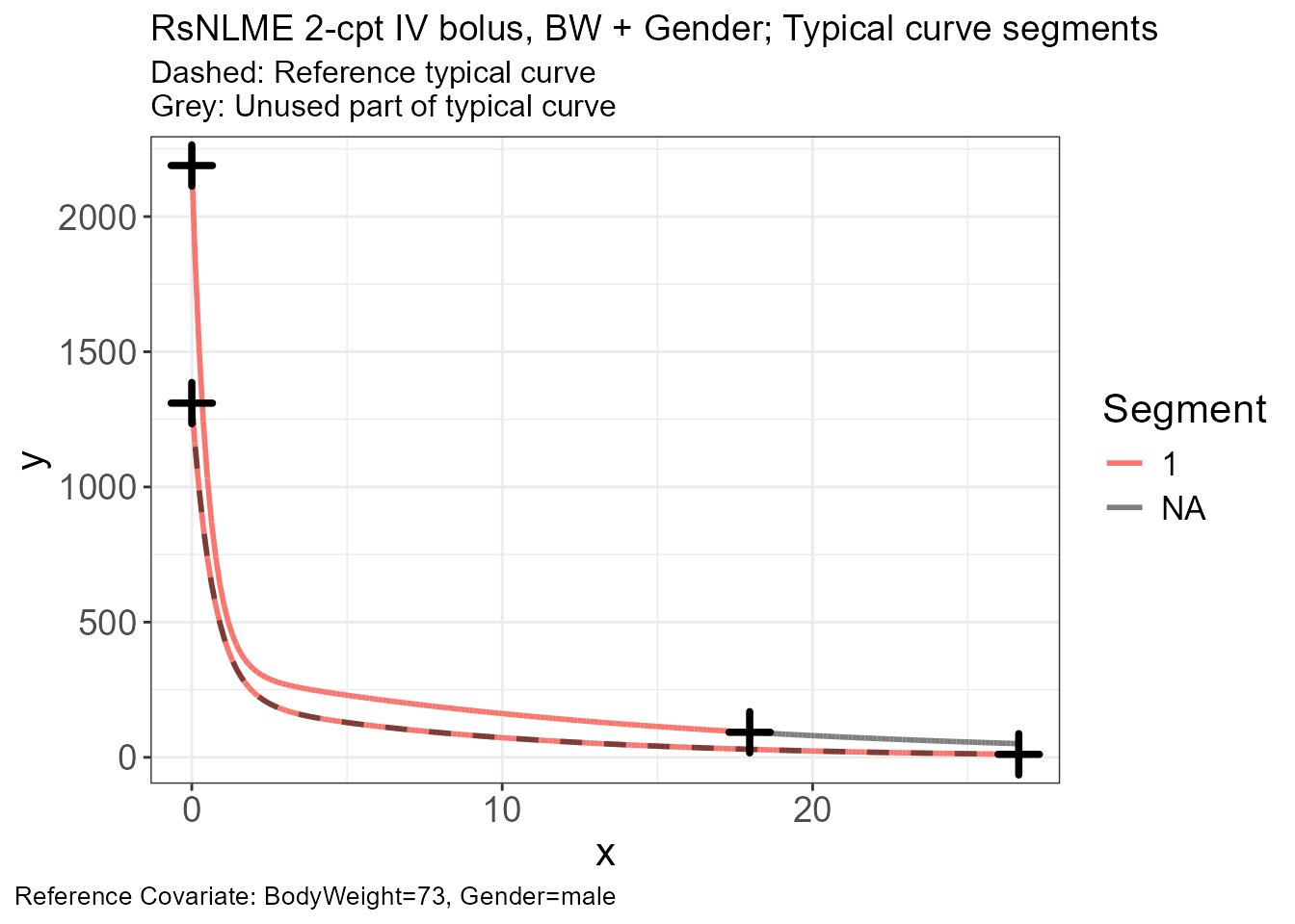
p.scaled.typical.full.curves.landmarks(vd)

p.scaling.factor(vd)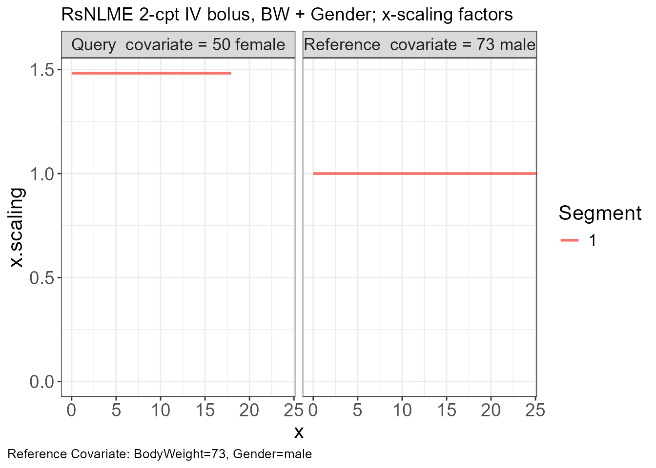

p.scaled.typical.curves(vd)

The full obs, typ, and sim datasets built earlier still work as direct inputs to vachette_data(); the filter above is purely for visual clarity. To compare additional covariate combinations, just add more rows to keep_combos.

6. Compare traditional VPC vs. vachette-transformed VPC

vd$obs.all and vd$sim.all carry both the original axes (x, y) and the vachette-transformed axes (x.scaled, y.scaled). Pass either set to tidyvpc to compare a binned VPC on the original axes to one on the vachette-aligned axes.

obs_trans <- vd$obs.all
sim_trans <- vd$sim.all

t_centers <- c(0.25, 1, 2, 4, 8, 16, 24)

vpc_traditional <- observed(obs_trans, x = x, y = y) |>
  simulated(sim_trans, x = x, y = y) |>
  binning(bin = "centers", centers = t_centers) |>
  vpcstats()

vpc_vachette <- observed(obs_trans, x = x.scaled, y = y.scaled) |>
  simulated(sim_trans, x = x.scaled, y = y.scaled) |>
  binning(bin = "centers", centers = t_centers) |>
  vpcstats()

plot(vpc_traditional) +
  labs(title = "Traditional VPC", x = "Time (h)", y = "Concentration")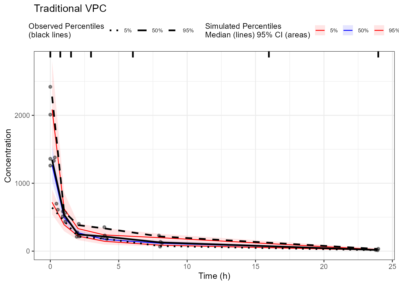


plot(vpc_vachette) +
  labs(title = "Vachette-transformed VPC",
       x = "Scaled time", y = "Scaled concentration")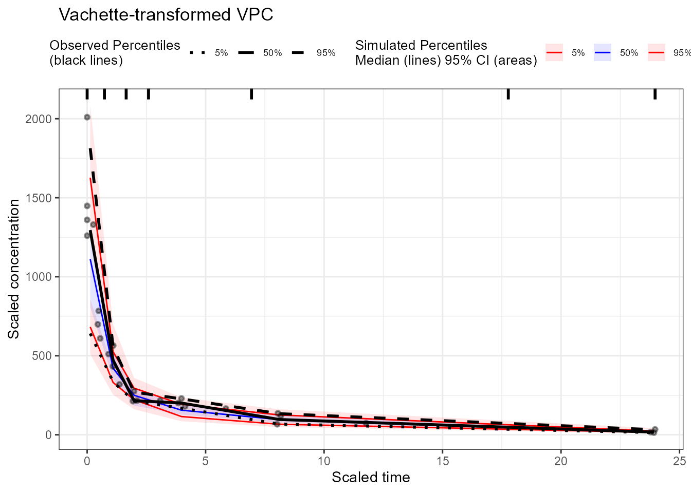

Recap

The pattern generalizes to any RsNLME covariate model:

Fit the model.
Use simmodel() with tableParams(variablesList = c(<observation>, <covariates...>), keepSource = TRUE) for sim.data.
Build a synthetic input dataset of (unique covariate combinations × dense time grid), freeze IIV via randomEffect(isFrozen = TRUE, value = 0), and run simmodel() with tableParams(variablesList = c(<concentration>, <covariates...>)) for typ.data.
Use the original input dataset (or predcheck0 from vpcmodel()) for obs.data.
Pass the three datasets to vachette_data() and apply transformations.