Using Model Builder in RStudio
modelbuilder_rstudio.RmdThe purpose of this vignette is to demonstrate how to utilize the
Certara.RsNLME.ModelBuilder R package to build and
parameterize NLME models from the Shiny GUI. In the following examples,
you will learn how to:
- Use the
modelBuilderUI()function to launch the Shiny GUI and create a built-in model involving covariates and BQL - Update values for fixed effects from the Shiny GUI using the
estimatesUI()function from theCertara.RsNLMEpackage - Fit the model in RStudio
- Copy and update the model with initial values set to be final parameter estimates
- Use the
modelTextual()function to directly edit PML statements from the Shiny GUI and return the updated model to RStudio - Fit the updated model
Data
We will be using the built-in pkcovbqlData from the
Certara.RsNLME package.
library(Certara.RsNLME)

pkcovbqlData <- Certara.RsNLME::pkcovbqlData

head(pkcovbqlData)
#> # A tibble: 6 × 8
#>      ID  Time  Dose  CObs  LLOQ CObsBQL    BW   PMA
#>   <dbl> <dbl> <dbl> <dbl> <dbl>   <dbl> <dbl> <dbl>
#> 1     1   0    1200  NA    0.01       0    12     1
#> 2     1   0.5    NA  97.7  0.01       0    12     1
#> 3     1   1      NA  97.4  0.01       0    12     1
#> 4     1   2      NA  79.5  0.01       0    12     1
#> 5     1   4      NA  96.4  0.01       0    12     1
#> 6     1   8      NA  87.2  0.01       0    12     1
Launch Model Builder (built-in model)
We will use the modelBuilderUI() function to launch the
Shiny GUI and build our model. Note that we will provide the
pkcovbqlData data.frame from above to the
data argument, and supply a string to the
modelName argument, which is used to create the run folder
for the associated output files from model execution.
library(Certara.RsNLME.ModelBuilder)

baseModel <- modelBuilderUI(data = pkcovbqlData, modelName = "baseModel")
Specify BQL
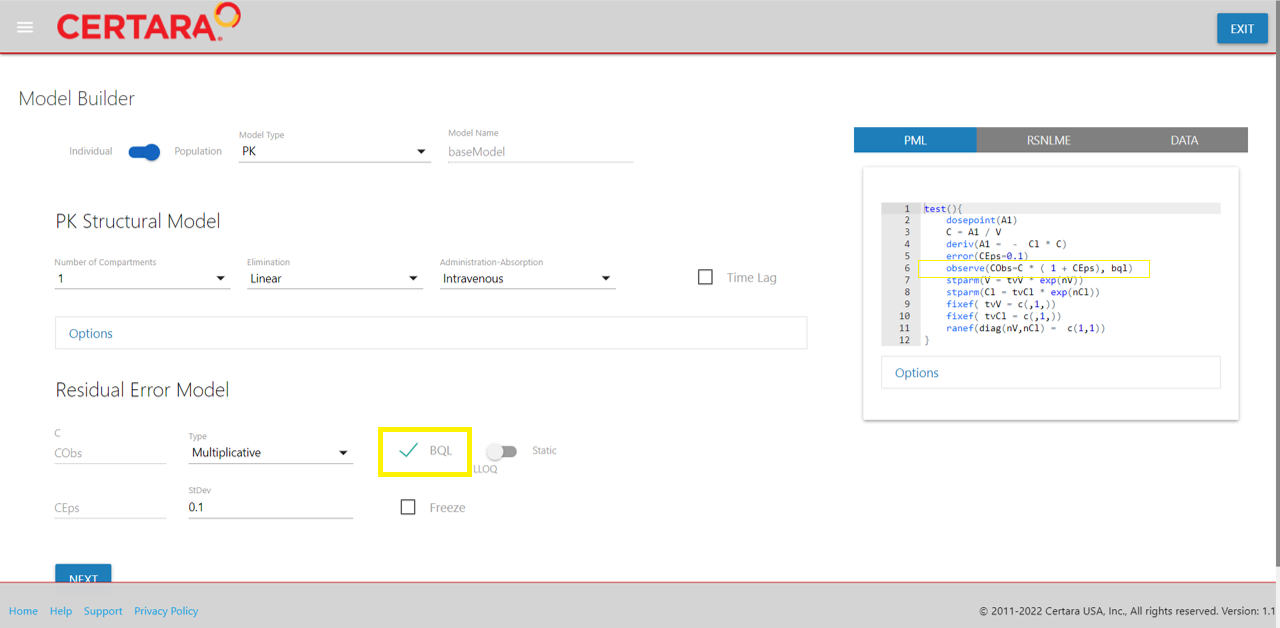
We will leave all options in the “PK Structural Model” section as default.
In the “Residual Error Model” selection, we will select the “BQL
checkbox.” This will add the bql indicator to line 6 in our
PML (e.g., observe(CObs=C * ( 1 + CEps), bql)).
Add covariates
Navigate to the “Parameters” tab, where you will see options related to “Structural Parameters,” “Covariates,” “Fixed Effects,” and “Random Effects.”
From the “Covariates” tab, we will introduce our two covariates into the model by clicking the “+” button, specifying the covariate type and whether to introduce the covariate effect on a structural parameter.
For our continuous covariate body weight, denoted as BW,
we will center the covariate on a value of 30 (or alternatively, select
“mean” or “median” to use as the centering value), and set the covariate
effect on our structural parameters, V and
Cl.
For our second (continuous) covariate PMA, we will add it to our
model without explicitly specifying the covariate effect at this time
(which will add the fcovariate(PMA) statement into PML code
without changing the stparm() statement).
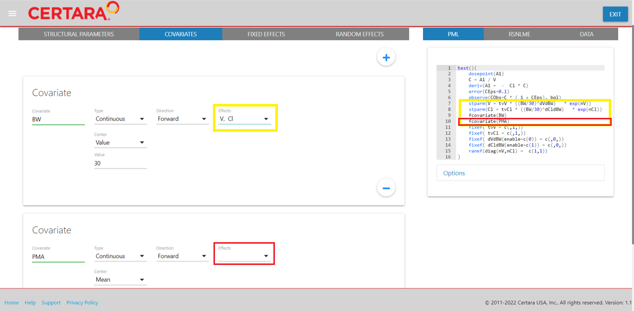
After adding the covariates into our model from the GUI, we can observe the corresponding updates to the PML on lines 7-10.
Update covariance matrices for random effects
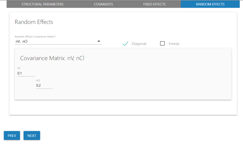
Next, from the “Random Effects” tab, select from the available ETA to
update one or more covariance matrices. We will specify values of 0.1
for nV and 0.2 for nCl.
Map model variables to columns
We will skip the input options step and navigate to the final step in
the Shiny GUI, “Column Mapping.” Here we will map all required model
variables to their corresponding columns in the input data. Columns
denoted with * are required.
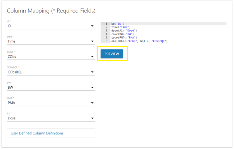
Clicking the “Preview” button (not required) will allow you to inspect the corresponding column definition file used by NLME during execution, ensuring all required model variables have been mapped correctly.
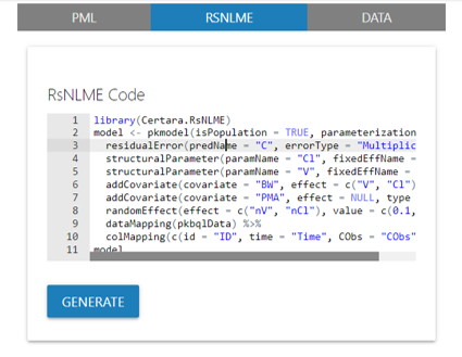
Generate RsNLME code
Whether you have finished building your model, or have more to do, at any time you may navigate to the “RsNLME” tab and click “Generate” to produce the corresponding RsNLME R code given the model-building operations you have performed in the GUI. This will allow you to recreate the model from the command line in future R sessions or share the model with other stakeholders to reproduce results.
Copy the RsNLME code generated in the Shiny GUI to a .R
and/or .Rmd script, where you can recreate and update the
model from the R command line.
library(Certara.RsNLME)
library(magrittr)

baseModel <- pkmodel(isPopulation = TRUE, parameterization = "Clearance", absorption = "Intravenous", numCompartments = 1, isClosedForm = FALSE, isTlag = FALSE, hasEliminationComp = FALSE, isFractionExcreted = FALSE, isSaturating = FALSE, infusionAllowed = FALSE, isDuration = FALSE, columnMap = FALSE, modelName = "baseModel") %>%
  residualError(predName = "C", errorType = "Multiplicative", SD = 0.1, isFrozen = FALSE, isBQL = TRUE) %>%
  structuralParameter(paramName = "Cl", fixedEffName = "tvCl", randomEffName = "nCl", style = "LogNormal", hasRandomEffect = TRUE) %>%
  structuralParameter(paramName = "V", fixedEffName = "tvV", randomEffName = "nV", style = "LogNormal", hasRandomEffect = TRUE) %>%
  addCovariate(covariate = "BW", effect = c("V", "Cl"), type = "Continuous", direction = "Forward", center = "Value", centerValue = 30L) %>%
  addCovariate(covariate = "PMA", effect = NULL, type = "Continuous", direction = "Forward", center = "Mean") %>%
  randomEffect(effect = c("nV", "nCl"), value = c(0.1, 0.2), isDiagonal = TRUE, isFrozen = FALSE) %>%
  dataMapping(pkcovbqlData) %>%
  colMapping(c(id = "ID", time = "Time", CObs = "CObs", CObsBQL = "CObsBQL", BW = "BW", PMA = "PMA", A1 = "Dose"))
Exit Model Builder
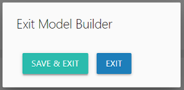
Clicking “Save & Exit” in the top-right of the screen will bring up the exit window. Selecting “Save & Exit” will return the RsNLME model object back to your R environment, ready for execution. Alternatively, selecting “Exit” will return to your R environment without saving your model.
Update initial values for fixed effects
You may update initial values for fixed effects from the “Fixed
Effects” tab in the modelBuilderUI() GUI, or alternatively,
use the estimatesUI()
function from Certara.RsNLME to visually determine a set of
reasonable initial values for fixed effects.
library(Certara.RsNLME)

baseModel <- estimatesUI(baseModel)
We will set the following values for fixed effects given evaluation of fit in the corresponding plot.
-
tvV= 20 -
tvCl= 8 -
dVdBW= 1 -
dCldBW= 1
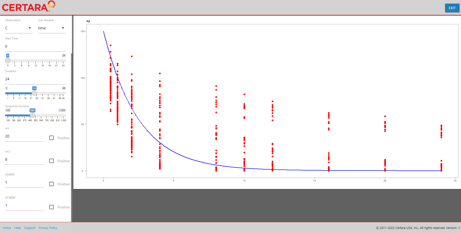
If you are unsure where to start with your fixed effects estimates, you can select the “Fit” button to generate baseline estimates. You can stick with the estimates provided or continue to fine tune them.
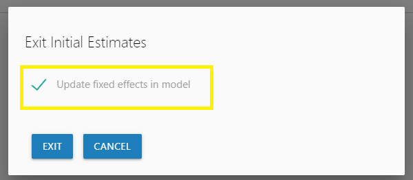
Click the “Save & Exit” button to accept the initial estimates and update the model object in your R environment or exit without saving to return to R without updating initial estimates for your model.

We can print() the model and see the updated values for
our fixed effects.
print(baseModel)
#>
#>  Model Overview
#>  -------------------------------------------
#> Model Name        :  baseModel
#> Working Directory :  C:/Users/mtalley/GitHub/R-RsNLME-model-builder/vignettes/baseModel
#> Is population     :  TRUE
#> Model Type        :  PK
#>
#>  PK
#>  -------------------------------------------
#> Parameterization  :  Clearance
#> Absorption        :  Intravenous
#> Num Compartments  :  1
#> Dose Tlag?        :  FALSE
#> Elimination Comp ?:  FALSE
#> Infusion Allowed ?:  FALSE
#> Sequential        :  FALSE
#> Freeze PK         :  FALSE
#>
#>  PML
#>  -------------------------------------------
#> test(){
#>     dosepoint(A1)
#>     C = A1 / V
#>     deriv(A1 =  -  Cl * C)
#>     error(CEps=0.1)
#>     observe(CObs=C * ( 1 + CEps), bql)
#>     stparm(V = tvV * ((BW/30)^dVdBW)   * exp(nV))
#>     stparm(Cl = tvCl * ((BW/30)^dCldBW)   * exp(nCl))
#>     fcovariate(BW)
#>     fcovariate(PMA)
#>     fixef( tvV = c(,20,))
#>     fixef( tvCl = c(,8,))
#>     fixef( dVdBW(enable=c(0)) = c(,1,))
#>     fixef( dCldBW(enable=c(1)) = c(,1,))
#>     ranef(diag(nV,nCl) = c(0.1,0.2))
#> }
#>
#>  Structural Parameters
#>  -------------------------------------------
#>  V Cl
#>  -------------------------------------------
#> Observations:
#> Observation Name :  CObs
#> Effect Name      :  C
#> Epsilon Name     :  CEps
#> Epsilon Type     :  Multiplicative
#> Epsilon frozen   :  FALSE
#> is BQL           :  TRUE
#>  -------------------------------------------
#>  Column Mappings
#>  -------------------------------------------
#> Model Variable Name : Data Column name
#> id                  : ID
#> time                : Time
#> A1                  : Dose
#> BW                  : BW
#> PMA                 : PMA
#> CObs                : CObs
#> CObsBQL             : CObsBQL
Fit the initial model
Now that we’ve defined appropriate values for our fixed effects, we
will fit the model in RStudio using the function fitmodel()
from Certara.RsNLME.
library(Certara.RsNLME)

baseJob <- fitmodel(baseModel)
#> Using MPI host with 4 cores
#>
#> NLME Job
#> sharedDirectory is not given in the host class instance.
#> Valid NLME_ROOT_DIRECTORY is not given, using current working directory:
#> C:/Users/mtalley/GitHub/R-RsNLME-model-builder/vignettes
#>
#> Compiling 1 of 1 NLME models
#> TDL5 version: 24.9.2.1
#>
#> Status: OK
#> License expires: 2026-08-06
#> Refresh until: 2025-09-04 22:16:52
#> Current Date: 2025-08-05
#> The model compiled
#>
#>
#>  Iteration    -2LL     tvV    tvCl    dVdBW  dCldBW nSubj nObs
#>          1 2642.96 23.8689 8.18440 0.902166 1.28015    80  800
#>          2 2615.21 24.3689 8.19965 0.842822 1.38964    80  800
#>          3 2545.31 26.1404 8.22741 0.560995 1.91161    80  800
#>          4 2494.21 24.3861 8.17291 0.799068 1.92974    80  800
#>          5 2472.67 24.7155 8.08545 0.835674 2.13684    80  800
#>          6 2457.11 24.6638 8.04369 0.781643 2.18438    80  800
#>          7 2455.28 25.0976 8.01678 0.771658 2.17206    80  800
#>          8 2453.26 24.5998 7.90991 0.751189 2.14356    80  800
#>          9 2448.66 24.7020 7.79512 0.741226 2.18738    80  800
#>         10 2441.66 24.9085 7.61638 0.754266 2.21733    80  800
#>         11 2437.08 24.9018 7.33681 0.766579 2.24009    80  800
#>         12 2435.11 24.8010 7.63493 0.766938 2.21619    80  800
#>         13 2434.73 24.7721 7.68259 0.764938 2.22005    80  800
#>         14 2434.71 24.7723 7.71752 0.765022 2.22053    80  800
#>         15 2434.71 24.7724 7.71725 0.765006 2.22040    80  800
#>         16 2434.71 24.7724 7.71714 0.765000 2.22038    80  800
#>         17 2434.71 24.7748 7.71650 0.764909 2.21936    80  800
#>         18 2434.71 24.7784 7.71702 0.764971 2.21954    80  800
#>         19 2434.71 24.7765 7.71832 0.765035 2.21934    80  800
#>         20 2434.71 24.7772 7.72025 0.765100 2.21947    80  800
#>
#> Trying to generate job results...
#>
#> Generating Overall.csv
#> Generating EtaEta.csv
#> Generating EtaCov.csv
#> Generating EtaCovariate.csv
#> Generating EtaCovariateCat.csv
#> Generating StrCovariate.csv
#> Generating Eta.csv
#> Generating EtaStacked.csv
#> Generating bluptable.dat
#> Generating ConvergenceData.csv
#> Generating initest.csv
#> Generating doses.csv
#> Generating omega.csv
#> Generating omega_stderr.csv
#> Generating theta.csv
#> Generating thetaCorrelation.csv
#> Generating thetaCovariance.csv
#> Generating Covariance.csv
#> Generating Residuals.csv
#> Generating posthoc.csv
#>
#> Finished summarizing results. Transferring data and loading the results...
#> Done generating job results.

print(baseJob$Overall)
#>    Scenario RetCode    LogLik     -2LL      AIC      BIC nParm  nObs  nSub
#>      <char>   <int>     <num>    <num>    <num>    <num> <int> <int> <int>
#> 1: WorkFlow       1 -1217.353 2434.706 2448.706 2481.498     7   800    80
#>    EpsShrinkage Condition
#>           <num>     <num>
#> 1:      0.10531  26.51068
Copy model and accept parameter estimates
After fitting our initial model, we will create a new model using the
copyModel()
function and set the argument acceptAllEffects = TRUE to
accept the parameter estimates from our model run.
finalModel <- copyModel(baseModel, acceptAllEffects = TRUE, modelName = "finalModel")Edit/Update model
Models can be updated in one of two ways; using the
modelTextualUI() function from the
Certara.RsNLME.ModelBuilder package, or by relaunching
modelBuilderUI().
Editing with modelTextualUI()
We can make changes to the PML code for our model from the Shiny GUI
that is launched with modelTextualUI().
Functionality includes:
- Real time syntax check for PML code
- Add/edit column mapping specifications
- Add additional input options such as ADDL and steady state
library(Certara.RsNLME.ModelBuilder)

model <- modelTextualUI(finalModel)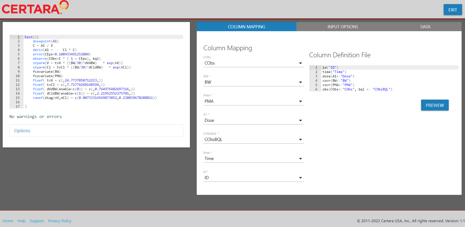
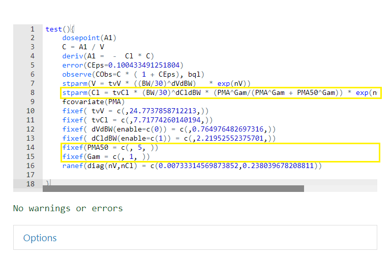
To incorporate the effect of PMA on the structural parameter Cl, we will change the following statement:
stparm(Cl = tvCl * ((BW/30)^dCldBW) * exp(nCl))
to
stparm(Cl = tvCl * (BW/30)^dCldBW * (PMA^Gam/(PMA^Gam + PMA50^Gam)) * exp(nCl))
Then add the following statements (right before the
ranef statement) to define the newly introduced fixed
effects.
fixef(PMA50 = c(, 5, ))
fixef(Gam = c(, 1, ))
Editing with modelBuilderUI()
In addition to creating models from scratch, the
modelBuilderUI() function also accepts model objects that
have already been created using the baseModel argument.
modelBuilderUI(baseModel = finalModel)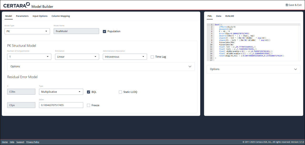
You will notice that all of the fixed and random effects in the PML code are those generated by our fitting of the model. This handy feature allows you to easily make changes to a model that is in progress without needing to start back at the beginning.
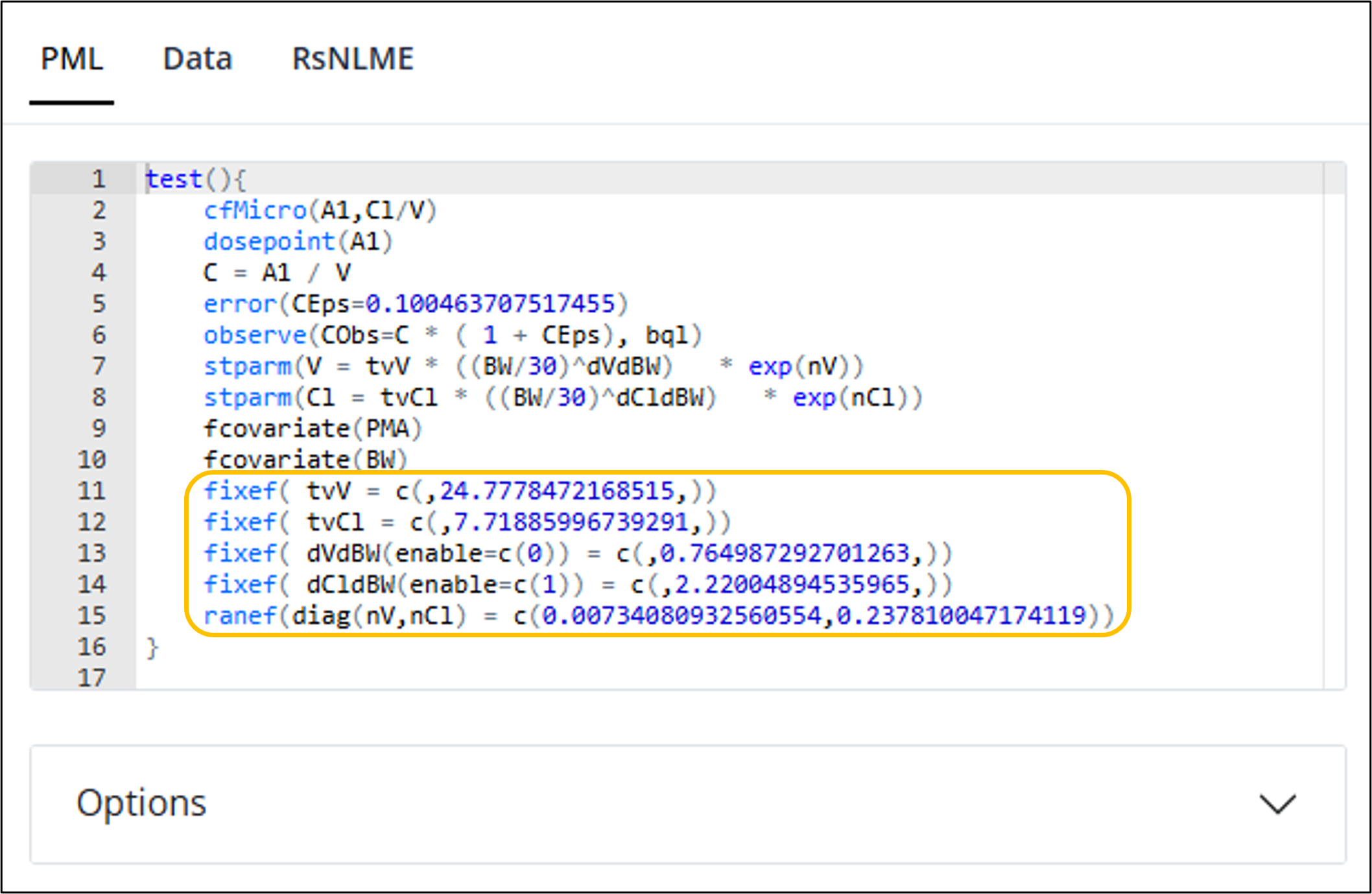
This feature is only available for non-textual models that have
not been modified with modelTextualUI().
Fit final model
After introducing the covariate effect of PMA to our structural
parameter, Cl, and adding our additional fixed effects, we
will fit the final model in RStudio once more using the function fitmodel()
from Certara.RsNLME.
library(Certara.RsNLME)

finalJob <- fitmodel(finalModel)
#> Using MPI host with 4 cores
#>
#> NLME Job
#> sharedDirectory is not given in the host class instance.
#> Valid NLME_ROOT_DIRECTORY is not given, using current working directory:
#> C:/Users/mtalley/GitHub/R-RsNLME-model-builder/vignettes
#>
#> Compiling 1 of 1 NLME models
#> TDL5 version: 24.9.2.1
#>
#> Status: OK
#> License expires: 2026-08-06
#> Refresh until: 2025-09-04 22:16:52
#> Current Date: 2025-08-05
#> The model compiled
#>
#>
#>  Iteration    -2LL     tvV    tvCl    dVdBW  dCldBW nSubj nObs
#>          1 2434.72 24.8045 7.72902 0.765058 2.22198    80  800
#>          2 2434.71 24.7987 7.72899 0.765049 2.22194    80  800
#>          3 2434.71 24.7722 7.72861 0.764998 2.22164    80  800
#>          4 2434.71 24.7736 7.72853 0.764998 2.22160    80  800
#>          5 2434.71 24.7735 7.72484 0.764793 2.21979    80  800
#>          6 2434.71 24.7725 7.72263 0.764783 2.21920    80  800
#>          7 2434.71 24.7786 7.71952 0.764999 2.21884    80  800
#>          8 2434.71 24.7772 7.72322 0.764966 2.21941    80  800
#>
#> Trying to generate job results...
#>
#> Generating Overall.csv
#> Generating EtaEta.csv
#> Generating EtaCov.csv
#> Generating EtaCovariate.csv
#> Generating EtaCovariateCat.csv
#> Generating StrCovariate.csv
#> Generating Eta.csv
#> Generating EtaStacked.csv
#> Generating bluptable.dat
#> Generating ConvergenceData.csv
#> Generating initest.csv
#> Generating doses.csv
#> Generating omega.csv
#> Generating omega_stderr.csv
#> Generating theta.csv
#> Generating thetaCorrelation.csv
#> Generating thetaCovariance.csv
#> Generating Covariance.csv
#> Generating Residuals.csv
#> Generating posthoc.csv
#>
#> Finished summarizing results. Transferring data and loading the results...
#> Done generating job results.

print(finalJob$Overall)
#>    Scenario RetCode    LogLik     -2LL      AIC      BIC nParm  nObs  nSub
#>      <char>   <int>     <num>    <num>    <num>    <num> <int> <int> <int>
#> 1: WorkFlow       1 -1217.353 2434.706 2448.706 2481.498     7   800    80
#>    EpsShrinkage Condition
#>           <num>     <num>
#> 1:      0.10536  26.45824