Using Model Builder in RStudio for Textual Models

In the following examples, you will learn how to:

Read the input dataset and mdl file (a file for PML model with .mdl extension) into RStudio
Use the textualModel() function from Certara.RsNLME to create a textual model object in your R environment
Launch the textual model editor using modelTextualUI(), map required columns, and specify covariate levels/labels

Data and model

The mdl and data, covariate.mdl and covariate.csv, are from Certara University’s (201-OD) Intermediate Population Modeling using Phoenix NLME. Both example files are distributed with the Certara.RsNLME.ModelBuilder package.

Import data

dataPath <- system.file("extdata", "covariate_data.csv", package = "Certara.RsNLME.ModelBuilder")

data <- read.csv(dataPath)

str(data)
#> 'data.frame':    511 obs. of  11 variables:
#>  $ ID    : int  1001 1001 1001 1001 1001 1001 1001 1001 1001 1001 ...
#>  $ PT    : int  1001 1001 1001 1001 1001 1001 1001 1001 1001 1001 ...
#>  $ TIME  : num  0 0.0486 0.0729 0.142 6.92 13.9 20.9 23 55 56.1 ...
#>  $ CONC  : num  0 6.11 5.59 5.12 2.37 ...
#>  $ DOSE  : num  25410 0 0 0 0 ...
#>  $ RATE  : int  0 0 0 0 0 0 0 0 0 0 ...
#>  $ E     : int  1 0 0 0 0 0 0 0 0 1 ...
#>  $ M     : int  1 0 0 0 0 0 0 0 0 1 ...
#>  $ CMT   : int  2 2 2 2 2 2 2 2 2 2 ...
#>  $ WEIGHT: num  77 77 77 77 77 77 77 77 77 77 ...
#>  $ SEX   : chr  "male" "male" "male" "male" ...

Import `.mdl`

mdlPath <- system.file("extdata", "covariate.mdl", package = "Certara.RsNLME.ModelBuilder", mustWork = TRUE)

mdl <- readLines(mdlPath)

cat(gsub(pattern = "\t", "\n\t", mdl))
#> test(){ 
#>  deriv(A1 = - Cl * C - Cl2 * (C - C2)) 
#>  deriv(A2 = Cl2 * (C - C2)) 
#>  dosepoint(A1, idosevar = A1Dose) 
#>  C = A1 / V 
#>  C2 = A2 / V2 
#>  error(CEps = 0.1) 
#>  observe(CObs = C * (1 + CEps)) 
#>  stparm(V = tvV * exp(nV)) 
#>  stparm(V2 = tvV2 * exp(nV2)) 
#>  stparm(Cl = tvCl * exp(nCl)) 
#>  stparm(Cl2 = tvCl2 * exp(nCl2)) 
#>  fcovariate(WEIGHT) 
#>  fcovariate(SEX()) 
#>  fixef(tvV = c(, 3739, )) 
#>  fixef(tvV2 = c(, 2852, )) 
#>  fixef(tvCl = c(, 210, )) 
#>  fixef(tvCl2 = c(, 897, )) 
#>  secondary(Ke = tvCl/tvV) 
#>  secondary(K12 = tvCl2/tvV) 
#>  secondary(K21 = tvCl2/tvV2) 
#>  secondary(r1 = ((K12+K21+Ke)^2-4*K21*Ke)^0.5) 
#>  secondary(Alpha = 0.5*(K12+K21+Ke+r1)) 
#>  secondary(Beta = 0.5*((K12+K21+Ke)-r1)) 
#>  secondary(A = (A1Dose/tvV*(Alpha-K21))/(Alpha-Beta)) 
#>  secondary(B = (-(A1Dose/tvV)*(Beta-K21))/(Alpha-Beta)) 
#>  secondary(AUC = A/Alpha+B/Beta) 
#>  secondary(Cmax = A1Dose/tvV) 
#>  secondary(AUMC = A/(Alpha*Alpha)+B/(Beta*Beta)) 
#>  secondary(MRT = AUMC/AUC) 
#>  secondary(VSS = tvCl*MRT) 
#>  secondary(Ke_hl = log(2)/Ke) 
#>  secondary(Alpha_hl = log(2)/Alpha) 
#>  secondary(Beta_hl = log(2)/Beta) 
#>  ranef(diag(nV, nCl, nV2, nCl2) = c(1, 1, 1, 1)) }

Create model object

Using the data in our R environment and the path to our .mdl file, we can create a textual model object inside RStudio using the textualmodel() function from the Certara.RsNLME package, then pass that model to the model argument of the modelTextualUI() function from Certara.RsNLME.ModelBuilder.


model <- textualmodel(modelName = "covariate", data = data, mdl = mdlPath)
#> Warning in checkCatCovariateMappingColumn(map, inputData, foundColumn,
#> modelTermName@variableName): The corresponding data column SEX for covariate
#> SEX is of class character. Please specify the name and the associated value for
#> each category through 'addLabel' function

print(model)
#> 
#>  Model Overview 
#>  ------------------------------------------- 
#> Model Name        :  covariate
#> Working Directory :  C:/Users/jcraig/Documents/GitHub/R-RsNLME-model-builder/vignettes/covariate
#> Model Type        :  Textual
#> 
#>  PML 
#>  ------------------------------------------- 
#> test(){
#>  deriv(A1 = - Cl * C - Cl2 * (C - C2))
#>  deriv(A2 = Cl2 * (C - C2))
#>  dosepoint(A1, idosevar = A1Dose)
#>  C = A1 / V
#>  C2 = A2 / V2
#>  error(CEps = 0.1)
#>  observe(CObs = C * (1 + CEps))
#>  stparm(V = tvV * exp(nV))
#>  stparm(V2 = tvV2 * exp(nV2))
#>  stparm(Cl = tvCl * exp(nCl))
#>  stparm(Cl2 = tvCl2 * exp(nCl2))
#>  fcovariate(WEIGHT)
#>  fcovariate(SEX())
#>  fixef(tvV = c(, 3739, ))
#>  fixef(tvV2 = c(, 2852, ))
#>  fixef(tvCl = c(, 210, ))
#>  fixef(tvCl2 = c(, 897, ))
#>  secondary(Ke = tvCl/tvV)
#>  secondary(K12 = tvCl2/tvV)
#>  secondary(K21 = tvCl2/tvV2)
#>  secondary(r1 = ((K12+K21+Ke)^2-4*K21*Ke)^0.5)
#>  secondary(Alpha = 0.5*(K12+K21+Ke+r1))
#>  secondary(Beta = 0.5*((K12+K21+Ke)-r1))
#>  secondary(A = (A1Dose/tvV*(Alpha-K21))/(Alpha-Beta))
#>  secondary(B = (-(A1Dose/tvV)*(Beta-K21))/(Alpha-Beta))
#>  secondary(AUC = A/Alpha+B/Beta)
#>  secondary(Cmax = A1Dose/tvV)
#>  secondary(AUMC = A/(Alpha*Alpha)+B/(Beta*Beta))
#>  secondary(MRT = AUMC/AUC)
#>  secondary(VSS = tvCl*MRT)
#>  secondary(Ke_hl = log(2)/Ke)
#>  secondary(Alpha_hl = log(2)/Alpha)
#>  secondary(Beta_hl = log(2)/Beta)
#>  ranef(diag(nV, nCl, nV2, nCl2) = c(1, 1, 1, 1))
#> }
#> 
#>  Structural Parameters 
#>  ------------------------------------------- 
#>  V V2 Cl Cl2
#>  ------------------------------------------- 
#>  Column Mappings 
#>  ------------------------------------------- 
#> Model Variable Name : Data Column name
#> id                  : ID
#> time                : TIME
#> A1                  : ?
#> WEIGHT              : WEIGHT
#> SEX                 : SEX
#> CObs                : ?

We can see that the columns in our data that share the same name as model variables get automatically mapped. We also received a warning about required covariate labels for our categorical covariate SEX, which is of class chr in the data.

unique(data$SEX)
#> [1] "male"   "female"

Map variables to columns through textual model builder

We can use the modelTextualUI() function to map the remaining columns and add corresponding levels/labels for our categorical covariate SEX.


model <- modelTextualUI(model)

After initializing the Shiny interface, we can see the PML editor on the left of the page, and various options related to column mapping on the right.

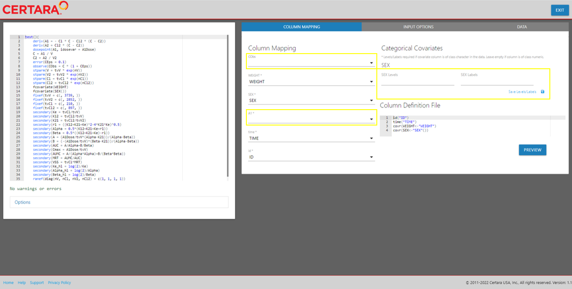
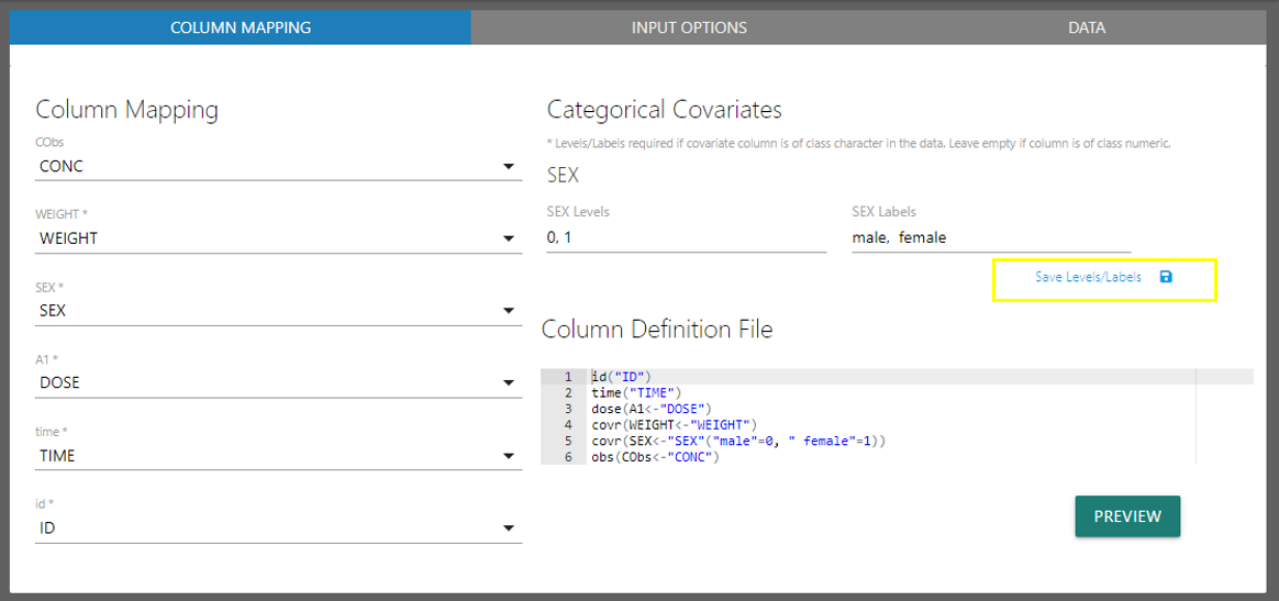
We will need to populate the blank inputs in the above screenshot. Select available columns in the input data from the dropdown inputs to map corresponding model variables. If categorical covariates exist in your model, you will see corresponding “Levels” and “Labels” inputs are displayed in the UI.

If the covariate column is class character in the data, you must specify these inputs and the click “Save Levels/Labels”. Leave empty if the covariate is already encoded as numeric.

Data and model

Import data

Import .mdl

Create model object

Map variables to columns through textual model builder

Import `.mdl`