Quantitative Predictive Check (QPC) scoring for VPC

Introduction

A Visual Predictive Check (VPC) is typically assessed visually by checking:

calibration (are observations inside simulated prediction intervals?)
bias and trend (does the model systematically miss in certain x regions?)
sharpness (are prediction intervals unnecessarily wide?)

The Quantitative Predictive Check (QPC) score in tidyvpc is a numeric summary of these features, computed from an existing tidyvpcobj after vpcstats().

QPC produces a table qpc.stats and a composite scalar qpc_score (lower is better) that can be used for automated model comparison and optimization.

What QPC measures (methodology overview)

QPC is computed from o$stats (the data.table produced by vpcstats()), which contains (for continuous VPCs) curve points across quantiles:

qname: quantile curve (e.g. q0.05, q0.5, q0.95)
y: observed curve value at x
md: simulated median curve at x
lo, hi: simulated confidence interval bounds at x for that quantile curve

At each curve point, QPC derives:

Coverage: whether $y \in [lo, hi]$
Deviation: $|y - md|$ relative to PI half-width
Drift: Spearman correlation of residuals $(y-md)$ versus x (monotonic bias)
Sharpness: interval width (penalizes “variance inflation”)
Proper interval score (Winkler): rewards narrow intervals but penalizes misses

These are aggregated across curves and combined into qpc_score with user-controlled weights.

Penalties (what is printed)

qpcstats() prints a scalar qpc_score plus a component breakdown. Each component is designed to be 0 = best and larger values = worse.

At a high level:

Coverage penalties measure calibration (are observed curves inside simulated uncertainty bands?).
MAE and drift penalties measure agreement and bias structure (how far and whether the residuals trend with x).
Sharpness and interval penalties discourage “variance inflation” (overly wide bands that can artificially increase coverage).

More concretely (continuous VPC):

Median coverage penalty (coverage_penalty_med): computed from the median quantile curve (the curve closest to $q=0.5$ ): $1 - \text{mean}(\mathbf{1}[y \in [lo,hi]])$ Lower is better; 0 means the observed median curve is always inside the simulated band.
Tail coverage penalty (coverage_penalty_tails): computed from the lowest and highest quantile curves available (typically $q=0.05$ and $q=0.95$ ), averaged: $\frac{(1-\text{coverage}_{low}) + (1-\text{coverage}_{high})}{2}$
MAE penalty (mae_penalty_all): based on deviation scaled by PI half-width: $dev\_mid = \frac{|y-md|}{(hi-lo)/2}$ then bounded to $[0,1]$ and averaged across curves. This highlights “large misses relative to the model’s own uncertainty”.
Drift penalty (rho_penalty_all): absolute Spearman correlation of residuals $(y-md)$ vs x (averaged across curves), bounded to $[0,1]$ . Values near 0 indicate no monotonic bias trend across x; larger values indicate systematic drift.
Sharpness penalty (sharpness_penalty): penalizes wide bands using relative width: $width\_{rel} = \frac{(hi-lo)}{|md|}$ By default (single-VPC scoring), this is mapped to $[0,1)$ with a bounded transform: $1 - e^{-\max(width\_{rel}, 0)}$ Optionally, you can anchor this with sharp_ref for cross-model comparability.
Interval penalty (interval_penalty): based on the Winkler interval score for nominal PI level $(1-\alpha)$ : $$ IS = (hi-lo) + \\frac{2}{\\alpha}(lo-y)\\mathbf{1}[y<lo] + \\frac{2}{\\alpha}(y-hi)\\mathbf{1}[y>hi] $$ This rewards narrow intervals but strongly penalizes misses. By default we apply a bounded transform to a normalized score; optionally you can anchor with interval_ref.

Finally:

$qpc\_score = \sum_i w_i \cdot penalty_i$

where w is the named weight vector (med_cov, tail_cov, mae, drift, sharp, interval).

Data

We’ll use the built-in tidyvpc::obs_data and tidyvpc::sim_data and follow the standard preprocessing used throughout our vignettes.

obs_data <- as.data.table(tidyvpc::obs_data)
sim_data <- as.data.table(tidyvpc::sim_data)

obs_data <- obs_data[MDV == 0]
sim_data <- sim_data[MDV == 0]

Add the population prediction PRED (from replicate 1) into the observed data for pcVPC examples:

obs_data$PRED <- sim_data[REP == 1, PRED]

Example 1: Basic QPC scoring

Below is a standard continuous VPC using binless VPC stats. The QPC computation is a post-processing step after vpcstats().

vpc <- observed(obs_data, x = TIME, y = DV) %>%
  simulated(sim_data, y = DV) %>%
  binless() %>%
  vpcstats()

vpc <- qpcstats(vpc)

print(vpc)
#> VPC with 100 replicates 
#> Stratified by:  
#> QPC: qpc_score = 0.159 (lower is better)
#> Breakdown (0 = best):
#>   median coverage penalty  0.000
#>   tail coverage penalty    0.092
#>   MAE penalty              0.221
#>   drift penalty            0.409
#>   sharpness penalty        0.272
#>   interval penalty         0.391
#> 
#>                x  qname         y        md        lo        hi
#>            <num> <fctr>     <num>     <num>     <num>     <num>
#>    1:  0.2157624  q0.05  20.27050  18.70099  15.46726  22.76529
#>    2:  0.4694366  q0.05  26.85172  24.20164  20.90806  28.69981
#>    3:  0.8271844  q0.05  36.13299  32.25889  27.80422  37.28306
#>    4:  1.7724895  q0.05  47.97810  45.68455  39.37618  51.15900
#>    5:  1.7142415  q0.05  48.59415  46.13059  39.92622  51.83491
#>   ---                                                          
#> 1646:  3.1146520  q0.95 187.64868 157.66057 135.21747 185.70608
#> 1647:  3.9526689  q0.95 162.26683 149.76519 128.25975 168.88196
#> 1648:  6.0247591  q0.95 119.55945 122.36560 105.29532 140.59213
#> 1649:  7.7967326  q0.95 103.60993 101.08928  88.41343 115.52899
#> 1650: 12.2981243  q0.95  63.09294  69.37852  61.51805  85.95328

The composite score is available in qpc.stats$qpc_score (for stratified VPCs you will also see an qpc_scope == "overall" row).

Plot the VPC:

plot(vpc)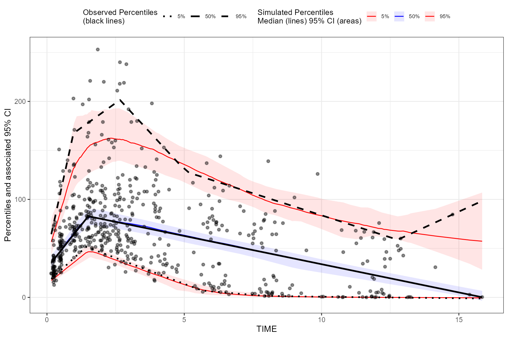

Example 2: QPC with prediction correction and stratification

QPC relies on vpc$stats, so it naturally works with prediction correction and stratification (for continuous VPCs).

vpc_pc_strat <- observed(obs_data, x = TIME, y = DV) %>%
  simulated(sim_data, y = DV) %>%
  stratify(STUDY ~ GENDER) %>%
  predcorrect(pred = PRED) %>%
  binless() %>%
  vpcstats()

vpc_pc_strat <- qpcstats(vpc_pc_strat)
print(vpc_pc_strat)
#> Prediction corrected VPC with 100 replicates 
#> Stratified by: STUDY, GENDER 
#> QPC: qpc_score = 0.148 (lower is better)
#> Breakdown (0 = best):
#>   median coverage penalty  0.009
#>   tail coverage penalty    0.037
#>   MAE penalty              0.201
#>   drift penalty            0.078
#>   sharpness penalty        0.453
#>   interval penalty         0.542
#> 
#> QPC qpc_score by stratum:
#>      STUDY  GENDER qpc_score qpc_scope
#>     <char>  <char>     <num>    <char>
#> 1: Study A       F 0.2185022   stratum
#> 2: Study B       F 0.1143301   stratum
#> 3: Study A       M 0.1760193   stratum
#> 4: Study B       M 0.1995141   stratum
#> 5: __ALL__ __ALL__ 0.1481005   overall
#>                x  qname   STUDY GENDER         y        md        lo       hi
#>            <num> <fctr>  <char> <char>     <num>     <num>     <num>    <num>
#>    1:  0.2414537  q0.05 Study A      F 22.628106 21.603303 14.635225 29.01338
#>    2:  0.6153070  q0.05 Study A      F 31.298883 31.217977 22.157131 43.88344
#>    3:  0.7493947  q0.05 Study A      F 34.408780 34.786598 25.021506 49.07117
#>    4:  1.6711424  q0.05 Study A      F 55.786869 59.999193 39.790871 82.52384
#>    5:  2.2418821  q0.05 Study A      F 69.024031 66.798270 45.272725 93.57229
#>   ---                                                                        
#> 1646:  2.9649190  q0.95 Study B      M 80.150799 75.984410 61.464186 97.94624
#> 1647:  4.2881855  q0.95 Study B      M 60.858937 58.079728 43.476314 75.06576
#> 1648:  6.0457983  q0.95 Study B      M 36.202388 34.662559 21.504472 51.58254
#> 1649:  7.9075620  q0.95 Study B      M 21.905414 20.454721 11.120393 34.17353
#> 1650: 12.0612380  q0.95 Study B      M  8.275706  6.636687  2.630895 14.68703

Plot the stratified pcVPC:

plot(vpc_pc_strat)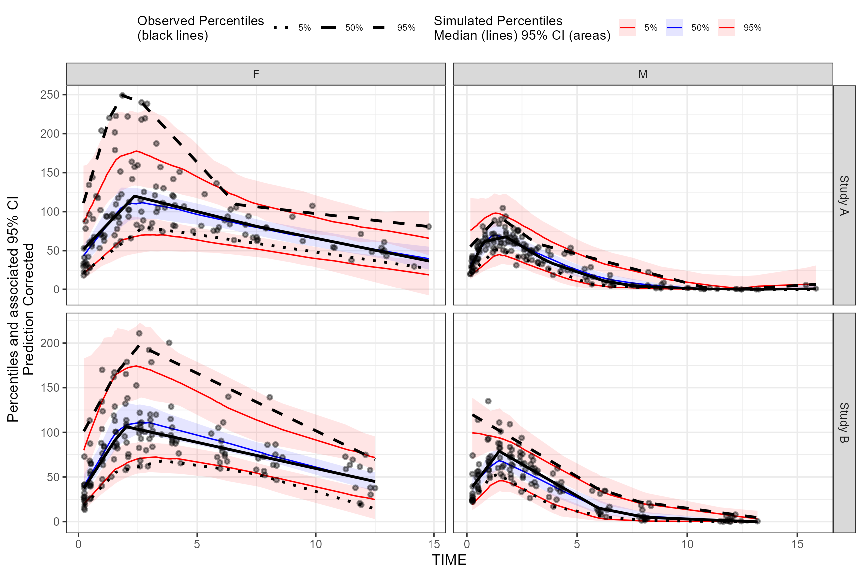

Interpreting differences between `vpc` and `vpc_pc_strat`

In the vignette examples you printed:

The prediction-corrected + stratified VPC (vpc_pc_strat) shows a lower drift penalty (residuals trend less with x), because prediction correction and stratification often remove structured bias that would otherwise appear as monotonic drift.
At the same time, vpc_pc_strat can show higher sharpness/interval penalties if the simulated uncertainty bands are wider within strata (or if prediction correction changes the scale/structure of residuals), because QPC explicitly penalizes overly wide intervals even when they improve coverage.
The per-stratum qpc_score table helps localize which subpopulations drive the overall score: strata with worse calibration (coverage penalties) or wider uncertainty (sharpness/interval penalties) will typically have higher qpc_score.

Example 3: QPC scoring with traditional binning()

QPC works with traditional binned VPCs as well (it scores directly from vpc$stats). The only difference is that vpcstats() will compute summaries at xbin instead of x.

vpc_binned <- observed(obs_data, x = TIME, y = DV) %>%
  simulated(sim_data, y = DV) %>%
  binning(bin = NTIME) %>%
  vpcstats()

vpc_binned <- qpcstats(vpc_binned)

print(vpc_binned)
#> VPC with 100 replicates 
#> Stratified by:  
#> QPC: qpc_score = 0.149 (lower is better)
#> Breakdown (0 = best):
#>   median coverage penalty  0.000
#>   tail coverage penalty    0.091
#>   MAE penalty              0.199
#>   drift penalty            0.276
#>   sharpness penalty        0.311
#>   interval penalty         0.428
#> 
#> Key: <xbin>
#>        bin       xbin  qname       y          lo          md          hi
#>     <fctr>      <num> <fctr>   <num>       <num>       <num>       <num>
#>  1:   0.25  0.2490835  q0.05 17.4250 13.20370500 16.63365000  20.0638487
#>  2:   0.25  0.2490835   q0.5 28.1000 26.33373750 30.44625000  36.4071750
#>  3:   0.25  0.2490835  q0.95 70.9100 47.45008250 55.05687500  71.2563250
#>  4:    0.5  0.5009004  q0.05 28.9200 24.25121000 29.00000000  35.0677837
#>  5:    0.5  0.5009004   q0.5 51.8000 46.10241250 51.90550000  60.0179125
#> ---                                                                     
#> 29:      8  8.0691507   q0.5 35.0000 24.03068750 33.87400000  42.8817250
#> 30:      8  8.0691507  q0.95 95.7900 83.68695000 96.48842500 110.8845750
#> 31:     12 12.0253628  q0.05  0.1291  0.02170331  0.08714695   0.2521808
#> 32:     12 12.0253628   q0.5 13.3750  7.52458375 15.91905000  24.0568625
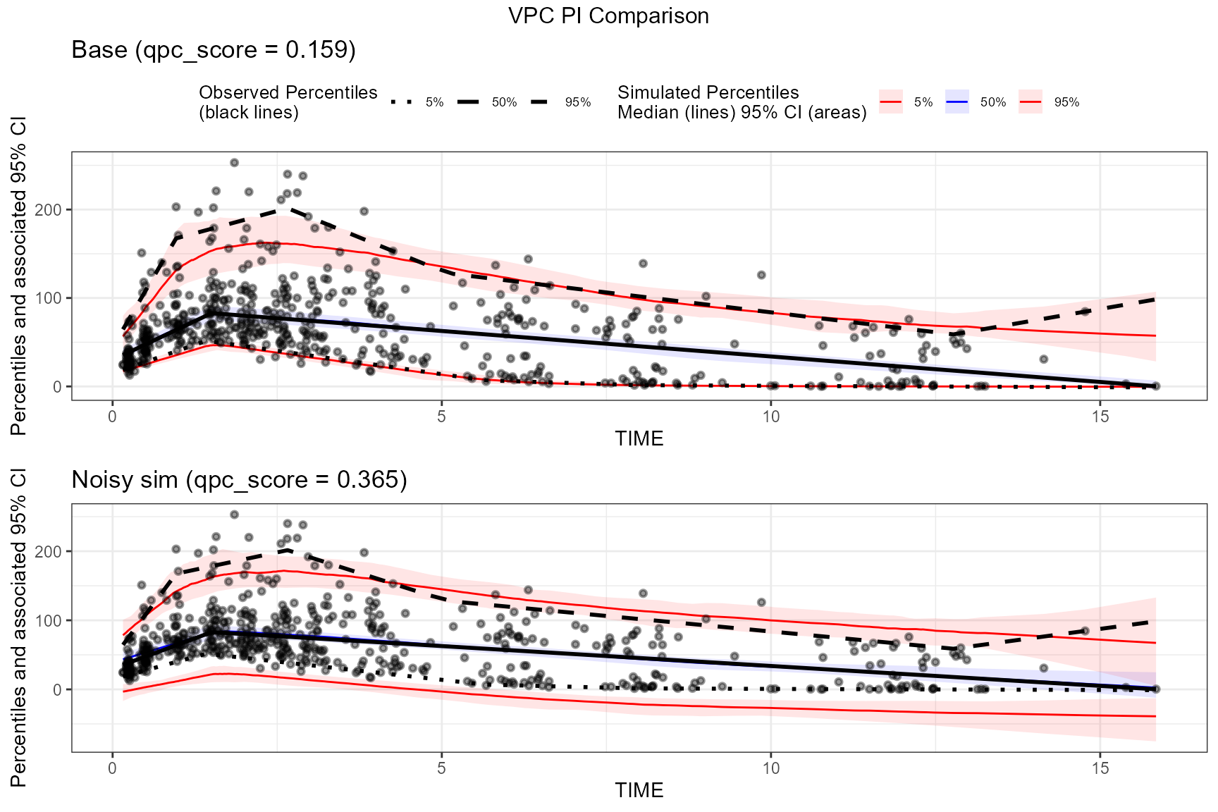
#> 33:     12 12.0253628  q0.95 67.5600 59.34408250 68.91725000  82.5615012

Example 4: Noisy simulations → wider confidence intervals → worse QPC

One failure mode of purely visual scoring is that very wide simulated confidence intervals can appear to “cover everything”. QPC penalizes this via sharpness and interval score components.

Here we artificially add noise to the simulated DV values to create wider confidence intervals, then compare qpc.stats.

sim_data_noisy <- copy(sim_data)

# Increase variability of simulated DV values; this should widen lo/hi bands.
sim_data_noisy[, DV := DV + rnorm(.N, mean = 0, sd = 25)]

vpc_base <- observed(obs_data, x = TIME, y = DV) %>%
  simulated(sim_data, y = DV) %>%
  binless() %>%
  vpcstats() %>%
  qpcstats()

vpc_noisy <- observed(obs_data, x = TIME, y = DV) %>%
  simulated(sim_data_noisy, y = DV) %>%
  binless() %>%
  vpcstats() %>%
  qpcstats()

base_overall <- vpc_base$qpc.stats[qpc_scope == "overall"]
noisy_overall <- vpc_noisy$qpc.stats[qpc_scope == "overall"]

cmp <- rbindlist(list(
  cbind(data.table(case = "base"), base_overall),
  cbind(data.table(case = "noisy_sim"), noisy_overall)
), fill = TRUE)

cmp_summary <- cmp[, .(
  Case = case,
  `QPC score` = qpc_score,
  `Median coverage` = coverage_penalty_med,
  `Tail coverage` = coverage_penalty_tails,
  Sharpness = sharpness_penalty,
  Interval = interval_penalty
)]

cmp_summary[, (names(cmp_summary)[-1]) := lapply(.SD, \(x) round(x, 3)), .SDcols = names(cmp_summary)[-1]]
knitr::kable(cmp_summary, caption = "QPC summary: baseline vs noisy simulations (0 = best; lower qpc_score is better)")

QPC summary: baseline vs noisy simulations (0 = best; lower qpc_score is better)
Case	QPC score	Median coverage	Tail coverage	Sharpness	Interval
base	0.159	0	0.092	0.272	0.391
noisy_sim	0.365	0	0.588	0.304	0.966

In this comparison you will typically see:

sharpness_penalty increases with wider prediction intervals
interval_penalty increases because the Winkler score increases with width (even if coverage improves)
therefore qpc_score tends to increase (worse)

Compare the two plots:

    qpc_base <- vpc_base$qpc.stats[qpc_scope == "overall", qpc_score][1]
qpc_noisy <- vpc_noisy$qpc.stats[qpc_scope == "overall", qpc_score][1]

p_base <- plot(vpc_base) +
  ggplot2::ggtitle(sprintf("Base (qpc_score = %.3f)", qpc_base))

p_noisy <- plot(vpc_noisy) +
  ggplot2::theme(legend.position = "none") +
  ggplot2::ggtitle(sprintf("Noisy sim (qpc_score = %.3f)", qpc_noisy))

egg::ggarrange(p_base,
               p_noisy,
               nrow = 2, ncol = 1,
               top = "VPC PI Comparison"
)

Tips for using `sharp_ref` and `interval_ref`

By default (sharp_ref = NULL, interval_ref = NULL), QPC uses self-normalizing bounded transforms so you can score a single VPC without external calibration.

If you are comparing many models (e.g. search/optimization) and need more stable cross-run comparability, set:

sharp_ref: a reference sharpness level (e.g. median across a model population)
interval_ref: a reference interval-score level (e.g. median/75th percentile across models)

vpc <- qpcstats(vpc, sharp_ref = 0.15, interval_ref = 2.5)