tidyvpc with nlmixr2

Introduction

tidyvpc and nlmixr2 can work together seamlessly. The information below will provide step-by-step methods for using tidyvpc to create visual predictive checks (VPCs) for nlmixr2 models.

Setup

R setup

First, you must load both libraries.

suppressPackageStartupMessages(library(tidyvpc, quietly = TRUE))
library(nlmixr2, quietly = TRUE)
library(magrittr)

Model fitting

Second, we will fit a simple model to use as an example. For more information on using nlmixr2 for model fitting, see the nlmixr2 website.

one_compartment <- function() {
  ini({
    tka <- log(1.57); label("Ka")
    tcl <- log(2.72); label("Cl")
    tv <- log(31.5); label("V")
    eta_ka ~ 0.6
    eta_cl ~ 0.3
    eta_v ~ 0.1
    add_sd <- 0.7
  })
  # and a model block with the error specification and model specification
  model({
    ka <- exp(tka + eta_ka)
    cl <- exp(tcl + eta_cl)
    v <- exp(tv + eta_v)
    d/dt(depot) <- -ka * depot
    d/dt(center) <- ka * depot - cl / v * center
    cp <- center / v
    cp ~ add(add_sd)
  })
}

data_model <- theo_sd
data_model$WTSTRATA <- ifelse(data_model$WT < median(data_model$WT), "Low weight", "High weight")

fit <- nlmixr2(one_compartment, data_model, est="saem", saemControl(print=0))
#> → loading into symengine environment...
#> → pruning branches (`if`/`else`) of saem model...
#> ✔ done
#> → finding duplicate expressions in saem model...
#> [====|====|====|====|====|====|====|====|====|====] 0:00:00
#> → optimizing duplicate expressions in saem model...
#> [====|====|====|====|====|====|====|====|====|====] 0:00:00
#> ✔ done
#> using C compiler: 'gcc.exe (x86_64-posix-seh, Built by strawberryperl.com project) 7.1.0'
#> rxode2 2.0.14 using 4 threads (see ?getRxThreads)
#>   no cache: create with `rxCreateCache()`
#> Calculating covariance matrix
#> → loading into symengine environment...
#> → pruning branches (`if`/`else`) of saem model...
#> ✔ done
#> → finding duplicate expressions in saem predOnly model 0...
#> → finding duplicate expressions in saem predOnly model 1...
#> → optimizing duplicate expressions in saem predOnly model 1...
#> → finding duplicate expressions in saem predOnly model 2...
#> ✔ done
#> using C compiler: 'gcc.exe (x86_64-posix-seh, Built by strawberryperl.com project) 7.1.0'
#> → Calculating residuals/tables
#> ✔ done
#> → compress origData in nlmixr2 object, save 7288
#> → compress phiM in nlmixr2 object, save 64048
#> → compress parHist in nlmixr2 object, save 9760
#> → compress saem0 in nlmixr2 object, save 28952

VPC preparation

nlmixr2 provides a method for simulating multiple studies to prepare for a VPC. Use the keep argument to add columns from the source data to the simulated output (e.g. to use it for stratification of the VPC).

fit_vpcsim <- vpcSim(object = fit, keep = "WTSTRATA")
#> using C compiler: 'gcc.exe (x86_64-posix-seh, Built by strawberryperl.com project) 7.1.0'

Following the vpcSim() call, the remainder of the steps use tidyvpc to generate the vpc.

Generate a standard VPC

The x and y arguments to observed() are the columns from your original dataset. The x and y arguments to simulated() will almost always be time and sim based on the outut from vpcSim().

obs_data <- data_model[data_model$EVID == 0,]

vpc <-
  observed(obs_data, x=TIME, y=DV) %>%
  simulated(fit_vpcsim, x=time, y=sim) %>%
  stratify(~ WTSTRATA) %>%
  binning(bin = "jenks") %>%
  vpcstats()

plot(vpc)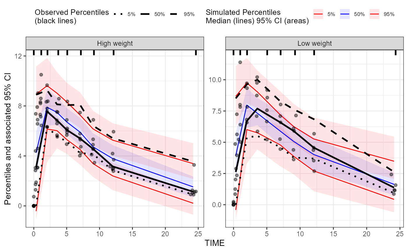

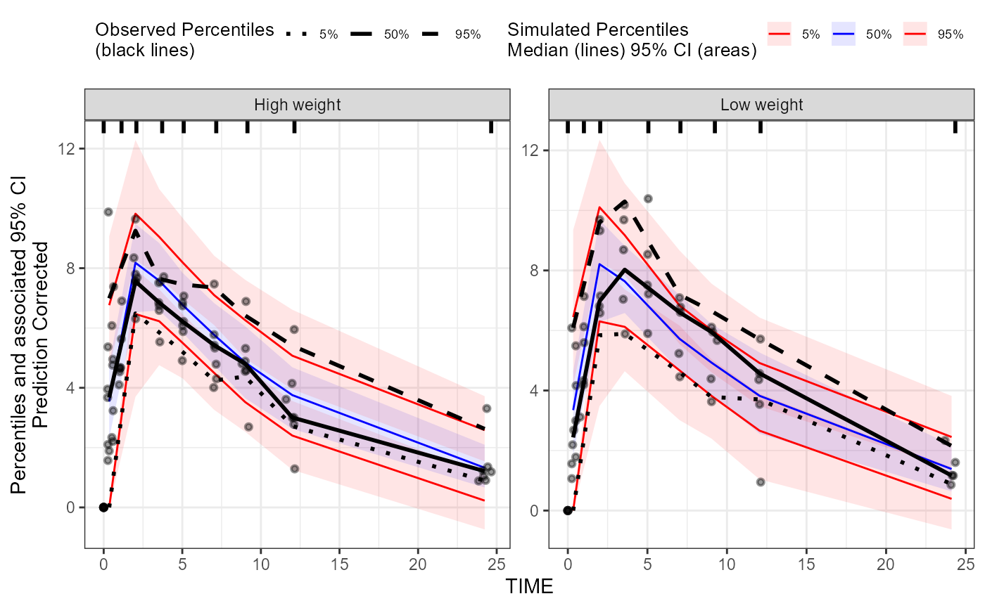
Prediction-corrected VPC

For a pred-corrected VPC, you need the population predicted value in the observed data. That is straight-forward to add with nlmixr2 by adding the predictions to all rows with EVID == 0.

# Add PRED to observed data
data_pred <- data_model[data_model$EVID == 0, ]
data_pred$PRED <- fit$PRED

vpc_predcorr <-
  observed(data_pred, x=TIME, y=DV) %>%
  simulated(fit_vpcsim, x=time, y=sim) %>%
  stratify(~ WTSTRATA) %>%
  binning(bin = "jenks") %>%
  predcorrect(pred=PRED) %>%
  vpcstats()

plot(vpc_predcorr)