Using Model Executor from RStudio • Certara.RsNLME.ModelExecutor

Overview

The Certara.RsNLME.ModelExecutor Shiny GUI can be used alongside Certara.RsNLME for a robust and efficient execution of RsNLME models. Specifically, users create models and hosts in R through the Certara.RsNLME package, and execute them using Certara.RsNLME.ModelExecutor, which allows users to choose different run modes and specify engine arguments in the Shiny GUI. All model execution results can be found in the working directory of the model.

Build base model

We’ll define a basic two-compartment population PK model with IV bolus as well as its associated column mappings through the Certara.RsNLME built-in function pkmodel(). The input data used in this example is the built-in pkData from the Certara.RsNLME package.

*Note: The corresponding R script used in this example can be found in RsNLME Example12

  baseModel <- pkmodel(numCompartments = 2, data = pkData,
                      ID = "Subject", Time = "Act_Time", A1 = "Amount", CObs = "Conc", 
                      modelName = "TwCpt_IVBolus_FOCE_ELS")

Next, we’ll update parameters in our model:

Disable the corresponding random effects for structural parameter V2
Change initial values for fixed effects, tvV, tvCl, tvV2, and tvCl2, to be 15, 5, 40, and 15, respectively
Change the covariance matrix of random effects, nV, nCl, and nCl2, to be a diagonal matrix with all its diagonal elements being 0.1
Change the standard deviation of residual error to be 0.2

  baseModel <- baseModel %>%
    structuralParameter(paramName = "V2", hasRandomEffect = FALSE) %>%
    fixedEffect(effect = c("tvV", "tvCl", "tvV2", "tvCl2"), value = c(15, 5, 40, 15)) %>%
    randomEffect(effect = c("nV", "nCl", "nCl2"), value = rep(0.1, 3)) %>%
    residualError(predName = "C", SD = 0.2)

Define hosts

We will create two NlmeParallelHost: one for local execution and the other for remote execution.

  host_local <- hostParams(sharedDirectory = Sys.getenv("NLME_ROOT_DIRECTORY"),
                                 parallelMethod = "LOCAL_MPI",
                                 hostName = "local",
                                 numCores = 4)

  host_remote <- hostParams(sharedDirectory = "/home/nlmeuser",
                                  parallelMethod = "TORQUE",
                                  hostName = "remote_torque",
                                  machineName = "192.168.15.21",
                                  userName = "nlmeuser", 
                                  userPassword = "password",
                                  hostType = "Linux",
                                  isLocal = FALSE,
                                  numCores = 4)

  hosts <- c(host_local, host_remote)

Fit base model through model executor

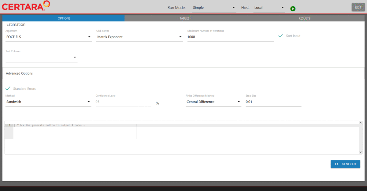
Run model executor using previously created model and hosts and execute the model with default setups

Note: The default values for the NLME engine arguments are chosen based on the default values of engineParams, type ?Certara.RsNLME::engineParams for details.

  modelExecutorUI(baseModel, hosts)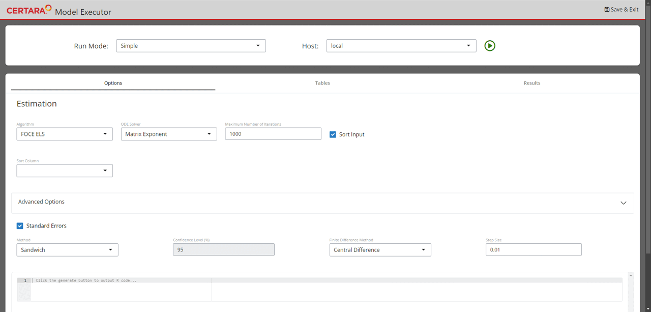

Since we didn’t provide the value of wd argument, results will be written to the current session’s working directory. For each execution, Model Executor creates a new directory with its name having the format nlme_shiny_typeOfRun_numOfSameTypeRunExecution. Since this is the first time that we run Model Executor to fit a model, results for this run can be found under the nlme_shiny_fitmodel_01 folder.

Real-time convergence plots

For the Simple run mode without any columns selected as Sort real-time convergence plots are being created. To observe those navigate to the Results tab (as shown on the above GIF) and switch to Convergence Plot subtab. Plots are being updated during execution and can be used to understand whether the process is converging and if there is a need to adjust execution setup

Add additional tables to be outputted

For the Simple run mode demonstrated above, one can click the “Add Table” button (located in the lower right corner of the page) to add any desired table to be outputted.

Build covariate model

After fitting the baseModel, let’s begin to introduce covariates. We will first copy our baseModel using the copyModel() function with acceptAllEffects set to TRUE to accept parameter estimates from our simple estimation run.

  ## Set the working directory of baseModel to the one returned by the model executor
  baseModel@modelInfo@workingDir <- paste0(getwd(), "/nlme_shiny_fitmodel_01")

  ## Copy the baseModel with acceptAllEffects = TRUE to accept parameter estimates from its simple estimation run 
  covariateModel <- copyModel(baseModel, acceptAllEffects = TRUE, 
                              modelName = "TwCpt_IVBolus_CovariateSearch")

Next, we’ll add the continuous covariate BodyWeight to our model and set the covariate effect on structural parameters V and Cl.

  covariateModel <- addCovariate(covariateModel,
                                 covariate = "BodyWeight",
                                 type = "Continuous",
                                 direction = "Backward",
                                 center = "Mean",
                                 effect = c("V", "Cl"))

Run stepwise covariate search for covariate model through model executor

Launch model executor again using the covariate model and hosts created above, choose Covariate search stepwise from the drop-down list of Run Mode (located in the top left corner of the page), and then run it.

  modelExecutorUI(covariateModel, hosts)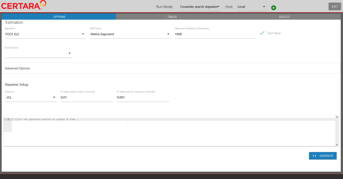

The stepwise.txt (which can be found in the nlme_shiny_stepwise_01 directory inside your session’s working directory) shows that the model selected by stepwise covariate search is the one with covariate BodyWeight having effect on both V and Cl.

Fit the selected model through model executor

We will fit the selected model through model executor. First, we will copy our covariateModel using the copyModel() function

  selectedCovariateModel <- copyModel(covariateModel,
                                      modelName = "TwCpt_IVBolus_selectedCovariateModel")

Next, we will launch model executor using the selectedCovariateModel and hosts created previously.

  modelExecutorUI(selectedCovariateModel, hosts)

Then, we will run it using the default setups. Note that this is the second time that the model executor is used to fit a model. Thus, the estimation results obtained for this run can be found in the nlme_shiny_fitmodel_02 folder.

Run VPC for the selected model through model executor

After fitting the selectedCovariateModel, we will run VPC for it. Again, we will first copy our selectedCovariateModel using the copyModel() function with acceptAllEffects set to TRUE to accept parameter estimates from our simple estimation run.

  ## Set the working directory of selectedCovariateModel to the one returned by the model executor
  selectedCovariateModel@modelInfo@workingDir <- paste0(getwd(), "/nlme_shiny_fitmodel_02") 

  ## Copy the selectedCovariateModel with acceptAllEffects = TRUE to accept parameter estimates from its simple estimation run
  vpcSelectedCovariateModel <- copyModel(selectedCovariateModel, 
                                         acceptAllEffects = TRUE, 
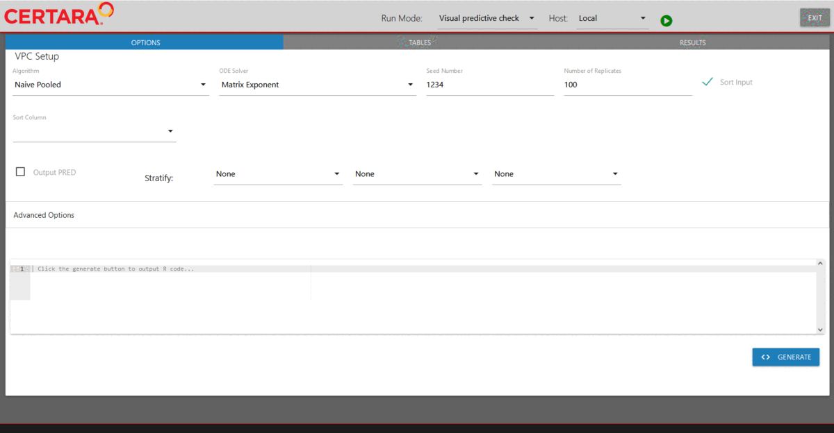
                                         modelName = "TwCpt_IVBolus_slectedCovariateModel_VPC")

Next, we will launch model executor using the above model and the hosts created previously. Then, we will choose Visual predictive check from the drop-down list of Run Mode (located in the top left corner of the page), add additional simulation tables if desired, and run it. Results of vpc run can be found under nlme_shiny_vpc_01 inside your session’s working directory.