Visualization of MOGA Results
moga_overview.RmdMulti-objective optimization (MOO) is an alternative approach to
optimization that permits subjective user input in the model selection
process. Rather than defining a single objective (e.g., fitness,
penalized -2ll), several objectives are optimized simultaneously. Model
selection within each iteration of the search is then based on
“non-dominated solutions”, which are models with the most optimized
objective values. After the search, the best non-dominated solutions
across all iterations are presented as a “final front” set of models.
This optimization method is available for implementation in Genetic
Algorithm (GA), resulting in the acronym “MOGA”. This vignette focuses
on how to visualize MOGA search results in
Certara.DarwinReporter. For more information on performing
MOO using Certara.RDarwin, click here.
Setup Search
We can use the same setup steps from the overview vignette to create our model object, but will need to modify the pyDarwin options for the MOGA algorithm.
optionSetup <- create_pyDarwinOptions(
  algorithm = "MOGA",   # Change to MOGA rather than GA
  num_generations = 10,
  population_size = 15,
  downhill_period = 0,
  local_2_bit_search = FALSE,
  final_downhill_search = FALSE,
  working_dir = getwd(),
  remove_temp_dir = FALSE
)
With our MOGA options created, we will write the
options.json, template.txt, and
tokens.json files before running the search.
# Write options.json file
write_pyDarwinOptions(pyDarwinOptions = optionSetup)

# Write template.txt file
write_ModelTemplateTokens(Description = "Search-numCpt-PeripherialRanef-3CovariatesOnClV-RSE",
                          Author = "Certara",
                          DataFilePath = "pkData.csv",
                          DataMapping = c(id = "Subject", time = "Act_Time", AMT = "Amount", CObs = "Conc", Age = "Age", BW = "BodyWeight", Sex = "Gender(female = 0, male = 1)"),
                          PMLParametersSets = models
                          )

# Run search
job <- run_pyDarwin(InterpreterPath = "C:/Program Files/Python311/python.exe", Wait = TRUE)
Model run output (click to hide)
[14:31:57] Model run priority is below_normal
[14:31:57] Using darwin.MemoryModelCache
[14:31:57] Writing intermediate output to C:/Darwin/output\results.csv
[14:31:57] Models will be saved in C:/Darwin\models.json
[14:31:57] Template file found at C:/Darwin/template.txt
[14:31:57] Tokens file found at C:/Darwin/tokens.json
[14:31:57] Algorithm: MOGA
[14:31:57] Engine: NLME
[14:31:57] Population size: 15
[14:31:57] num_generations: 10
[14:31:57] random_seed: 11
[14:31:57] use_effect_limit: False
[14:31:57] Project dir: C:\Darwin
[14:31:57] Data dir: C:\Darwin
[14:31:57] Project working dir: C:/Darwin
[14:31:57] Project temp dir: C:/Darwin\temp
[14:31:57] Project output dir: C:/Darwin/output
[14:31:57] Non-dominated models dir: C:/Darwin/non_dominated_models
[14:31:57] Search space size: 6144
[14:31:57] Estimated number of models to run: 150
[14:31:57] NLME found: C:/Program Files/Certara/NLME_Engine
[14:31:57] GCC found: C:/Program Files/Certara/mingw64
[14:31:57] Search start time: Tue Jul  1 14:31:57 2025
[14:31:57] Not using Post Run R code
[14:31:57] Not using Post Run Python code
[14:31:57] Checking files in C:\Darwin\temp\01\02
[14:32:06] Iteration =    01, Model     3,           Done,     OFV =  1535.010, NEP =  8,  message = No important warnings
[14:32:09] Iteration =    01, Model     4,           Done,     OFV =  1232.156, NEP = 12,  message = No important warnings
[14:32:09] Iteration =    01, Model     2,           Done,     OFV =  1228.000, NEP = 13,  message = No important warnings
[14:32:13] Iteration =    01, Model     1,           Done,     OFV =  1207.306, NEP = 15,  message = No important warnings
[14:32:19] Iteration =    01, Model     6,           Done,     OFV =  1624.296, NEP =  7,  message = No important warnings
[14:32:20] Iteration =    01, Model     7,           Done,     OFV =  1249.856, NEP = 13,  message = No important warnings
[14:32:23] Iteration =    01, Model     5,           Done,     OFV =  1223.552, NEP = 14,  message = No important warnings
[14:32:27] Iteration =    01, Model     8,           Done,     OFV =  1227.878, NEP = 12,  message = No important warnings
[14:32:32] Iteration =    01, Model     9,           Done,     OFV =  1232.560, NEP = 13,  message = No important warnings
[14:32:34] Iteration =    01, Model    10,           Done,     OFV =  1245.730, NEP = 11,  message = No important warnings
[14:32:34] Iteration =    01, Model    11,           Done,     OFV =  1252.674, NEP = 11,  message = No important warnings
[14:32:42] Iteration =    01, Model    12,           Done,     OFV =  1229.776, NEP = 13,  message = No important warnings
[14:32:43] Iteration =    01, Model    13,           Done,     OFV =  1221.906, NEP = 11,  message = No important warnings
[14:32:45] Iteration =    01, Model    15,           Done,     OFV =  1535.132, NEP =  9,  message = No important warnings
[14:32:46] Iteration =    01, Model    14,           Done,     OFV =  1217.216, NEP = 12,  message = No important warnings
[14:32:46] Current Non Dominated models:
[14:32:46] Model NLME_01_01.mmdl,  OFV =  1207.306, NEP = 15
[14:32:46] Model NLME_01_03.mmdl,  OFV =  1535.010, NEP =  8
[14:32:46] Model NLME_01_06.mmdl,  OFV =  1624.296, NEP =  7
[14:32:46] Model NLME_01_13.mmdl,  OFV =  1221.906, NEP = 11
[14:32:46] Model NLME_01_14.mmdl,  OFV =  1217.216, NEP = 12
[14:32:46] Time elapsed: 0.8 min.
[14:32:46] Estimated time remaining: 7.4 min.
...

[14:40:05] Current Non Dominated models:
[14:40:05] Model NLME_02_14.mmdl,  OFV =  1217.292, NEP = 11
[14:40:05] Model NLME_03_12.mmdl,  OFV =  1207.286, NEP = 15
[14:40:05] Model NLME_04_07.mmdl,  OFV =  1209.336, NEP = 14
[14:40:05] Model NLME_05_02.mmdl,  OFV =  1535.010, NEP =  7 (x2)
[14:40:05] Model NLME_05_08.mmdl,  OFV =  1221.906, NEP = 10
[14:40:05] Model NLME_06_10.mmdl,  OFV =  1215.954, NEP = 12
[14:40:05] Model NLME_07_01.mmdl,  OFV =  1674.356, NEP =  5 (x2)
[14:40:05] Model NLME_08_11.mmdl,  OFV =  1238.404, NEP =  8
[14:40:05] Model NLME_08_12.mmdl,  OFV =  1559.188, NEP =  6
[14:40:05] Model NLME_08_15.mmdl,  OFV =  1209.570, NEP = 13
[14:40:05] Model NLME_09_03.mmdl,  OFV =  1207.254, NEP = 16
[14:40:05] Model NLME_09_10.mmdl,  OFV =  1234.540, NEP =  9
[14:40:05] Model NLME_10_14.mmdl,  OFV =  1202.444, NEP = 18
[14:40:06]  MOGA best genome =
[[0 0 0 0 0 0 0 0 0 1 0 1 1]
 [0 0 0 0 0 0 0 0 0 1 0 1 0]
 [1 0 1 1 1 1 1 1 0 1 1 1 0]
 [0 0 0 1 1 0 0 0 0 0 0 1 1]
 [0 1 0 0 1 0 0 0 0 0 0 1 1]
 [0 0 0 1 0 0 0 0 0 0 1 1 1]
 [1 1 1 0 1 1 1 1 1 0 0 1 0]
 [0 1 0 0 1 0 0 1 1 0 0 1 0]
 [0 1 0 0 1 0 0 0 0 1 0 1 0]
 [0 1 0 1 1 1 0 1 1 0 0 1 0]
 [1 1 0 0 1 0 1 1 0 0 0 1 0]
 [0 1 1 0 1 0 0 1 0 1 0 1 1]
 [1 0 0 1 1 0 0 1 1 0 0 1 0]
 [1 1 0 0 1 1 1 1 1 0 0 1 0]
 [0 0 0 1 1 0 0 0 0 0 1 1 0]],
 OFV and # of parameters =
[[1674.356    5.   ]
 [1674.356    5.   ]
 [1202.444   18.   ]
 [1535.01     7.   ]
 [1238.404    8.   ]
 [1559.188    6.   ]
 [1207.254   16.   ]
 [1221.906   10.   ]
 [1234.54     9.   ]
 [1215.954   12.   ]
 [1209.57    13.   ]
 [1217.292   11.   ]
 [1209.336   14.   ]
 [1207.286   15.   ]
 [1535.01     7.   ]]
[14:40:06] Number of considered models: 150
[14:40:06] Number of models that were run during the search: 127
[14:40:06] Elapsed time: 8.1 minutes

[14:40:06] Search end time: Tue Jul  1 14:40:06 2025
Note: The above output is abbreviated. Only results from iteration 1 and final lines are displayed.
Get Results Overview
Now that we have our search results, we can bring them into our
environment and start to explore them. Results can be read in directly
using the non_dominated_models_dir argument in
darwin_data(), or by using the darwin_data()
and import_non_dominated_models() functions in
combination.
# Import search results
dir <- getwd()
nondom_dir <- paste0(dir, "/non_dominated_models")

model <- darwin_data(project_dir = dir, non_dominated_models_dir = nondom_dir)

# Or alternatively
model <- darwin_data(project_dir = dir) |>
  import_non_dominated_models(dir = nondom_dir)
We can check the results of ALL the models in the
search, or alternatively can use
summarise_overall_by_non_dominated_models() to generate a
quick overview of just the models selected to be in the final front. The
columns global_ff and moga_ff correlate to the
methods used to determine the final front models.
# Inspect all models from the search
head(model$non_dominated_models$final_front)

#> # A tibble: 6 × 9
#>   model_name   ofv   NEP    f1    f2 group         final_front global_ff moga_ff
#>   <chr>      <dbl> <int> <dbl> <int> <chr>         <lgl>       <lgl>     <lgl>
#> 1 NLME_01_03 1535.     8 1535.     8 non_dominated FALSE       FALSE     FALSE
#> 2 NLME_01_04 1232.    12 1232.    12 dominated     FALSE       FALSE     FALSE
#> 3 NLME_01_02 1228     13 1228     13 dominated     FALSE       FALSE     FALSE
#> 4 NLME_01_01 1207.    15 1207.    15 non_dominated FALSE       FALSE     FALSE
#> 5 NLME_01_06 1624.     7 1624.     7 non_dominated FALSE       FALSE     FALSE
#> 6 NLME_01_07 1250.    13 1250.    13 dominated     FALSE       FALSE     FALSE

# Inspect just the final front models
summarise_overall_by_non_dominated_models(model)

#> # A tibble: 13 × 15
#>    model_name RetCode `-2LL`   AIC   BIC nParm  nObs  nSub Condition   ofv   NEP    f1    f2 global_ff moga_ff
#>    <chr>        <int>  <dbl> <dbl> <dbl> <int> <int> <int>     <dbl> <dbl> <int> <dbl> <int> <lgl>     <lgl>
#>  1 NLME_02_14       1  1217. 1239. 1269.    11   112    16     83.9  1217.    11 1217.    11 TRUE      TRUE
#>  2 NLME_03_12       1  1207. 1237. 1278.    15   112    16     NA    1207.    15 1207.    15 TRUE      TRUE
#>  3 NLME_04_07       1  1209. 1237. 1275.    14   112    16   1321.   1209.    14 1209.    14 TRUE      TRUE
#>  4 NLME_05_02       1  1535. 1549. 1568.     7   112    16    321.   1535.     7 1535.     7 TRUE      TRUE
#>  5 NLME_05_08       1  1222. 1242. 1269.    10   112    16     NA    1222.    10 1222.    10 TRUE      TRUE
#>  6 NLME_06_10       1  1216. 1240. 1273.    12   112    16    367.   1216.    12 1216.    12 TRUE      TRUE
#>  7 NLME_07_01       1  1674. 1684. 1698.     5   112    16      4.87 1674.     5 1674.     5 TRUE      TRUE
#>  8 NLME_08_11       3  1238. 1254. 1276.     8   112    16      8.50 1238.     8 1238.     8 TRUE      TRUE
#>  9 NLME_08_12       1  1559. 1571. 1587.     6   112    16    223.   1559.     6 1559.     6 TRUE      TRUE
#> 10 NLME_08_15       1  1210. 1236. 1271.    13   112    16    923.   1210.    13 1210.    13 TRUE      TRUE
#> 11 NLME_09_03       1  1207. 1239. 1283.    16   112    16   1477.   1207.    16 1207.    16 TRUE      TRUE
#> 12 NLME_09_10       1  1235. 1253. 1277.     9   112    16      8.30 1235.     9 1235.     9 TRUE      TRUE
#> 13 NLME_10_14       1  1202. 1238. 1287.    18   112    16     NA    1202.    18 1202.    18 TRUE      TRUE
Models are originally placed in one of two classes; dominated and non-dominated. Non-dominated models are those selected by pyDarwin within each iteration of the search, while the selection for the final front can be decided in one of two ways.
Global Final Front
Models where global_ff is TRUE were
selected by the import_non_dominated_models() function
using the following two criteria. Are there any other models where:
- All objective values are less than or equal to those of the model of interest?
- At least one of the objective values is less than (i.e., better than) that objective value for the model of interest?
If a model has been deemed non-dominated by the pyDarwin search and there are no other models that meet both criteria, it is selected to be in the final front.
In the following example, we have two theoretical models selected as non-dominated during the pyDarwin search.
#>     Model   f1 f2
#> 1 Model 1 1000  8
#> 2 Model 2  800  8
We will start by looking at Model 1 as the model of interest:
- The objective values for Model 2 are both less than or equal to those of Model
- Additionally, at least one objective value (f1) for Model 2 is less than that of Model 1.
Because both criteria are satisfied, we can conclude that Model 2 dominates Model 1, therefore removing Model 1 from inclusion in the final front. Conversely, if we look at Model 2 as the model of interest, we will see that Model 1 is not able to satisfy both criteria, meaning Model 2 would be selected for the final front.
This method of model selection is considered more absolute, as it focuses purely on comparative objective values to select for the final front.
MOGA Final Front
Models where moga_ff is TRUE were selected
by the pyDarwin search using the above criteria, while also factoring in
additional crossover and mutation criteria. This method may be
considered more balanced, as it handles both objective values
along with additional search criteria.
While both methods will generally return the same results, certain model options can cause differences in the selected final front models. Retaining both classifications will give us more customization options in our downstream plotting and reports.
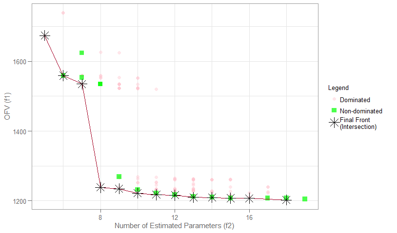
Plot Results
To better visualize the relationship between the models and their
objective values, we can plot them all using the
objectives_vs_non_dominated_models() function. The default
behavior of this function will return an interactive plotly
plot that we can explore data points with.
objectives_vs_non_dominated_models(darwin_data = model)If we want to customize the plot, we can change the colors used for
each group of models with the model_colors argument.
Additionally, we can turn this plot into a non-interactive
ggplot2 object using the interactive
argument.
objectives_vs_non_dominated_models(
  darwin_data = model,
  interactive = FALSE,
  model_colors = c(Dominated = "pink", `Non-dominated` = "green", `Final Front` = "black")
)
Explore Further with Shiny GUI
To really dig into the results of the pyDarwin search, launch the
Shiny GUI using darwinReportUI().
darwinReportUI(model)
You will recognize the plot on the overview page as the one we just
created using objectives_vs_non_dominated_models(), but
with even more cool features! At the top of the page you will find
filters for each objective. Adjusting these will update the plot and its
associated table below in real time.

While exploring the interactive plot, clicking on a point will
generate a pop-up window with useful model information. For final front
models, this modal includes the contents of the .mmdl file,
as well as a link to the diagnostics page to generate plots and tables
for the selected model.
From the diagnostics page, you can continue to customize your plots and tables, generate reproducible R code, and export your favorite diagnostics in organized reports!