DarwinReporter: A reporting toolkit for pyDarwin
DarwinReporter_Overview.RmdThe Certara.DarwinReporter package provides a Shiny
application, in addition to various plotting and data summary functions
for analyzing results of a pyDarwin automated model search.
This vignette provides an overview of an example R-based workflow for
performing an automated search with NLME using Certara.RDarwin
and analyzing results using the Certara.DarwinReporter
package.
Setup Search
We will be using a pharmacokinetic dataset containing 16 subjects
with single IV bolus dose for our search. The dataset is available
within the Certara.RsNLME package.
head(Certara.RsNLME::pkData)
#> # A tibble: 6 × 8
#>   Subject Nom_Time Act_Time Amount  Conc   Age BodyWeight Gender
#>     <dbl>    <dbl>    <dbl>  <dbl> <dbl> <dbl>      <dbl> <chr>
#> 1       1        0     0     25000  2010    22         73 male
#> 2       1        1     0.26     NA  1330    22         73 male
#> 3       1        1     1.1      NA   565    22         73 male
#> 4       1        2     2.1      NA   216    22         73 male
#> 5       1        4     4.13     NA   180    22         73 male
#> 6       1        8     8.17     NA   120    22         73 male
We will begin by writing this dataset to a csv file in our current working directory:
All candidate models assume linear elimination with parameterization set to “Clearance.” We will then search on:
Number of compartments: 1, 2, 3
Random effects for peripheral compartment parameters: V2, Cl2, V3, Cl3
Covariates: Age, BW, and Sex effect on Cl and V
Residual error model: Proportional or AdditiveMultiplicative
First, we will setup initial model sets to include 1, 2, and 3 compartments.
models <- get_PMLParametersSets(CompartmentsNumber = c(1, 2, 3))Let us view the models:
models
#> PK1IVC
#>  test() {
#>  cfMicro(A1, Cl / V)
#>  C = A1 / V
#>  dosepoint(A1, idosevar = A1Dose, infdosevar = A1InfDose, infratevar = A1InfRate)
#>  error(CEps = 0.1)
#>  observe(CObs = C * (1 + CEps))
#>
#>  stparm(Cl = tvCl * exp( nCl ))
#>  fixef(tvCl= c(, 1, ))
#>  ranef(diag(nCl) = c(1))
#>  stparm(V = tvV * exp( nV ))
#>  fixef(tvV= c(, 1, ))
#>  ranef(diag(nV) = c(1))
#>
#> }
#> PK2IVC
#>  test() {
#>  cfMicro(A1, Cl / V, Cl2 / V, Cl2 / V2)
#> C = A1 / V
#>  dosepoint(A1, idosevar = A1Dose, infdosevar = A1InfDose, infratevar = A1InfRate)
#>  error(CEps = 0.1)
#>  observe(CObs = C * (1 + CEps))
#>
#>  stparm(Cl = tvCl * exp( nCl ))
#>  fixef(tvCl= c(, 1, ))
#>  ranef(diag(nCl) = c(1))
#>  stparm(V = tvV * exp( nV ))
#>  fixef(tvV= c(, 1, ))
#>  ranef(diag(nV) = c(1))
#>  stparm(Cl2 = tvCl2 * exp( nCl2 ))
#>  fixef(tvCl2= c(, 1, ))
#>  ranef(diag(nCl2) = c(1))
#>  stparm(V2 = tvV2 * exp( nV2 ))
#>  fixef(tvV2= c(, 1, ))
#>  ranef(diag(nV2) = c(1))
#>
#> }
#> PK3IVC
#>  test() {
#>  cfMicro(A1, Cl / V, Cl2 / V, Cl2 / V2, Cl3 / V, Cl3 / V3)
#>  C = A1 / V
#>  dosepoint(A1, idosevar = A1Dose, infdosevar = A1InfDose, infratevar = A1InfRate)
#>  error(CEps = 0.1)
#>  observe(CObs = C * (1 + CEps))
#>
#>  stparm(Cl = tvCl * exp( nCl ))
#>  fixef(tvCl= c(, 1, ))
#>  ranef(diag(nCl) = c(1))
#>  stparm(V = tvV * exp( nV ))
#>  fixef(tvV= c(, 1, ))
#>  ranef(diag(nV) = c(1))
#>  stparm(Cl2 = tvCl2 * exp( nCl2 ))
#>  fixef(tvCl2= c(, 1, ))
#>  ranef(diag(nCl2) = c(1))
#>  stparm(V2 = tvV2 * exp( nV2 ))
#>  fixef(tvV2= c(, 1, ))
#>  ranef(diag(nV2) = c(1))
#>  stparm(Cl3 = tvCl3 * exp( nCl3 ))
#>  fixef(tvCl3= c(, 1, ))
#>  ranef(diag(nCl3) = c(1))
#>  stparm(V3 = tvV3 * exp( nV3 ))
#>  fixef(tvV3= c(, 1, ))
#>  ranef(diag(nV3) = c(1))
#>
#> }
Next, we will search whether peripheral compartment parameters, V2,
Cl2, V3, Cl3, have random effects by specifying the Name of
the random effect for corresponding structural parameter, and setting
the State argument to "Searched".
models <- models |>
  modify_Omega(Name = "nV2", State = "Searched") |>
  modify_Omega(Name = "nCl2", State = "Searched") |>
  modify_Omega(Name = "nV3", State = "Searched") |>
  modify_Omega(Name = "nCl3", State = "Searched")
Now, we will introduce a few covariates (Age, BW, and Sex) into the
search space in order to explore various covariate effects across
structural parameters V and Cl.
models <- models |>
  add_Covariate(Name = "Age", StParmNames = c("V", "Cl"), State = "Searched") |>
  add_Covariate(Name = "BW", StParmNames = c("V", "Cl"), State = "Searched", Center = 70) |>
  add_Covariate(Name = "Sex", Type = "Categorical", StParmNames = c("V", "Cl"), State = "Searched", Categories = c(0, 1))
Finally, we will add both a Proportional and Additive-Multiplicative
error model to the search space using the SigmasChosen
argument in the function modify_Observation():
models <- models |>
  modify_Observation(
    ObservationName = "CObs",
    SigmasChosen = Sigmas(
      AdditiveMultiplicative = list(PropPart = 0.1, AddPart = 0.01),
      Proportional = 0.1
    )
  )
Run Search
Before running the search, we first must configure a few options for
pyDarwin, such as the algorithm, number of generations/iterations
(num_generations), the number of models in each generation
(population_size), and the working_dir. For
this example, we will additionally perform a final downhill search after
the generations for GA have completed.
optionSetup <- create_pyDarwinOptions(
  algorithm = "GA",
  num_generations = 10,
  population_size = 10,
  downhill_period = 0,
  local_2_bit_search = FALSE,
  final_downhill_search = TRUE,
  working_dir = getwd(),
  remove_temp_dir = FALSE
)
Note, pyDarwin requires 3 input files for execution - template.txt, tokens.json, and options.json files. RDarwin provides functions to easily generate these files:
We will write the options.json file using values in our
optionSetup with the following command:
write_pyDarwinOptions(pyDarwinOptions = optionSetup)Similarly, we will write the template.txt file and
tokens.json file using the command below, passing the
models object we created to the
PMLParameterSets argument:
write_ModelTemplateTokens(Description = "Search-numCpt-PeripherialRanef-3CovariatesOnClV-RSE",
                          Author = "Certara",
                          DataFilePath = "pkData.csv",
                          DataMapping = c(id = "Subject", time = "Act_Time", AMT = "Amount", CObs = "Conc", Age = "Age", BW = "BodyWeight", Sex = "Gender(female = 0, male = 1)"),
                          PMLParametersSets = models
                          )
Note in the above command, we specified the path to our data file
using the DataFilePath argument and mapped required model
variables to column names in the data file using the
DataMapping argument. See
?Certara.RDarwin::get_ModelTermsToMap to list required
model variables for given search space.
Now we are ready to run the search.
job <- run_pyDarwin(InterpreterPath = "~/.venv/Scripts/python.exe", Wait = TRUE)[17:55:54] Model run priority is below_normal
[17:55:54] Using darwin.MemoryModelCache
[17:55:54] Writing intermediate output to C:/Workspace/Darwin/output\results.csv
[17:55:54] Models will be saved in C:/Workspace/Darwin\models.json
[17:55:54] Template file found at template.txt
[17:55:54] Tokens file found at tokens.json
[17:55:54] Algorithm: GA
[17:55:54] Engine: NLME
[17:55:54] random_seed: 11
[17:55:54] Project dir: C:\Workspace\Darwin
[17:55:54] Data dir: C:\Workspace\Darwin
[17:55:54] Project working dir: C:/Workspace/Darwin
[17:55:54] Project temp dir: C:/Workspace/Darwin\temp
[17:55:54] Project output dir: C:/Workspace/Darwin/output
[17:55:54] Key models dir: C:/Workspace/Darwin\key_models
[17:55:54] Search space size: 6144
[17:55:54] Estimated number of models to run: 230
[17:55:54] NLME found: C:/Program Files/Certara/NLME_Engine
[17:55:54] GCC found: C:/Program Files/Certara/mingw64
[17:55:54] Search start time: Tue Nov 14 17:55:54 2023
[17:55:54] Starting generation 1
[17:55:54] Not using Post Run R code
[17:55:54] Not using Post Run Python code
[17:55:54] Checking files in C:\Workspace\Darwin\temp\01\03
[17:56:19] Generation = 01, Model 3, Done, fitness = 1952.736, message = No important warnings
[17:56:21] Generation = 01, Model 4, Done, fitness = 1639.444, message = No important warnings
[17:56:28] Generation = 01, Model 1, Done, fitness = 1690.038, message = No important warnings
[17:56:35] Generation = 01, Model 2, Done, fitness = 1383.304, message = No important warnings
[17:56:49] Generation = 01, Model 5, Done, fitness = 1646.580, message = No important warnings
[17:56:51] Generation = 01, Model 6, Done, fitness = 1363.718, message = No important warnings
[17:56:52] Generation = 01, Model 7, Done, fitness = 1351.912, message = No important warnings
[17:57:05] Generation = 01, Model 8, Done, fitness = 1701.238, message = No important warnings
[17:57:07] Generation = 01, Model 9, Done, fitness = 1824.660, message = No important warnings
[17:57:15] Generation = 01, Model 10, Done, fitness = 1460.988, message = No important warnings
[17:57:15] Current generation best genome = [0, 1, 1, 0, 1, 1, 0, 0, 1, 1, 0, 0, 0], best fitness = 1351.9120
[17:57:15] Best overall fitness = 1351.912000, iteration 01, model 7
[17:57:15] No change in fitness for 1 generations, best fitness = 1351.9120
[17:57:15] Starting generation 2
[17:57:15] Time elapsed: 1.4 min.
[17:57:15] Estimated time remaining: 29 min.
...
[18:14:55] Done with final downhill step. best fitness = 1311.942
[18:14:55] Final output from best model is in C:/Workspace/Darwin/output\FinalResultFile.txt
[18:14:55] Number of considered models: 230
[18:14:55] Number of models that were run during the search: 141
[18:14:55] Number of unique models to best model: 91
[18:14:55] Time to best model: 12.2 minutes
[18:14:55] Best overall fitness: 1311.942000, iteration FND02, model 10
[18:14:55] Elapsed time: 19.0 minutes
[18:14:55] Search end time: Tue Nov 14 18:14:55 2023
[18:14:55] Key models:
[18:14:55] Generation = 01, Model 7, Done, fitness = 1351.912, message = No important warnings
[18:14:55] Generation = 04, Model 9, Done, fitness = 1338.992, message = No important warnings
[18:14:55] Generation = 05, Model 3, Done, fitness = 1334.540, message = No important warnings
[18:14:55] Generation = 06, Model 9, Done, fitness = 1324.540, message = No important warnings
[18:14:55] Generation = FND01, Model 8, Done, fitness = 1317.292, message = No important warnings
[18:14:55] Generation = FND02, Model 10, Done, fitness = 1311.942, message = No important warningsNote: The above output is abbreviated. Only results from generation 1 and final lines are displayed.
Analyze Results
We will use the function darwin_data() to import our
results into R:
ddb <- darwin_data(project_dir = getwd())We can plot fitness vs iteration:
fitness_vs_iteration(ddb)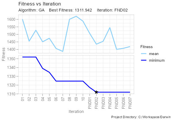
Or the penalty composition of min fitness by iteration:
fitness_penalties_vs_iteration(ddb, group_penalties = FALSE)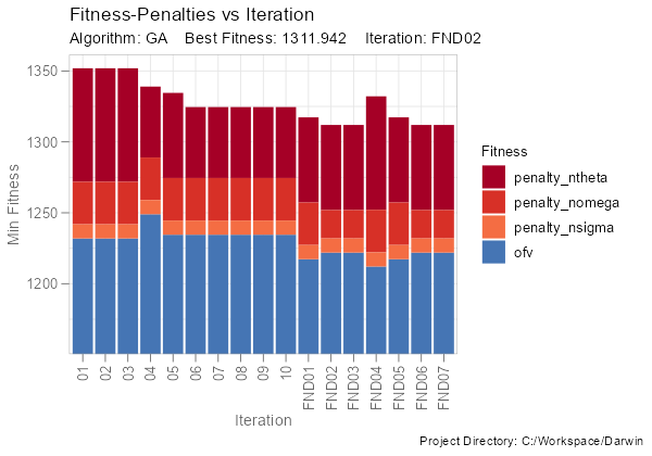
If we want to explore model diagnostic plots for key models, we can
use the function import_key_models(), specifying the path
to the “key_models” folder created by pyDarwin.
ddb <- ddb |>
  import_key_models(dir = file.path(getwd(), "key_models"))
Using the function darwinReportUI(), we can launch the
Shiny GUI and easily explore the search results.
darwinReportUI(ddb)
Within the application, users can explore model diagnostic plots across all key models, including the final model, create and customize GOF plots and tables, including generating the underlying R code to reproduce, and download R Markdown reports!