Paliperidone Palmitate Case Study

Overview

This Paliperidone Palmitate case study demonstrates a comprehensive Virtual Bioequivalence (VBE) analysis using the integrated Pirana-Simcyp^TM workflow. This study stems from an FDA grant and showcases the complete VBE process from initial setup through final statistical analysis.

The case study evaluates bioequivalence between reference and test formulations of Paliperidone Palmitate, focusing on the Critical Quality Attribute (CQA) of particle size distribution (PSD) mean radius. The analysis demonstrates how varying PSD parameters affects bioavailability and bioequivalence outcomes.

Key Objectives

• Demonstrate the complete VBE workflow using Pirana’s integrated tools
• Evaluate the impact of particle size distribution on bioequivalence
• Perform comprehensive statistical analysis including power, type I error, and safe space assessment
• Showcase the iterative nature of VBE analysis

Study Design

Critical Quality Attribute (CQA)

The primary CQA for this study is the Particle Size Distribution (PSD) Mean Radius. This parameter directly influences drug dissolution and absorption, making it critical for bioequivalence assessment.

Formulation Parameters

Parameter	Reference Value	Test Range	Units
PSD Mean Radius	4.6357	1.80 - 7.50	µm

Virtual Population Design

The study includes one reference formulation and multiple test formulations with varying PSD mean radius values:

PSD Mean Radius	Type	Number of Subjects	Description
4.6357	Reference	100,000	Reference formulation
1.8000	Test	2,500	Lower bound test
2.0000	Test	2,500	Lower bound test
2.6000	Test	2,500	Lower bound test
2.7762	Test	50,000	Type I error boundary
3.0000	Test	50,000	Lower range test
4.6357	Test	40,000	Perfect bioequivalence test
4.8375	Test	40,000	Upper range test
5.0679	Test	40,000	Upper range test
5.5000	Test	100,000	Upper range test
6.2300	Test	100,000	Upper range test
6.4500	Test	100,000	Upper range test
6.7000	Test	2,500	Upper bound test
6.8230	Test	50,000	Type I error boundary
7.1000	Test	2,500	Upper bound test
7.5000	Test	20,000	Upper bound test

Trial Design

The case study uses a parallel trial design. Currently, only parallel VBE trial designs are supported in the Pirana-Simcyp VBE module.

Simulation Performance

Estimated simulation run times across different subject numbers and available cores:

Number of Subjects	Number of Cores	Estimated Time (minutes)	Estimated Time (hours)
1,000	8	53.08	0.88
1,000	16	26.54	0.44
1,000	32	13.27	0.22
10,000	8	530.79	8.85
10,000	16	265.39	4.42
10,000	32	132.70	2.21
100,000	8	5,307.87	88.46
100,000	16	2,653.94	44.23
100,000	32	1,326.97	22.12

Setup and Configuration

Prerequisites

Note: Make sure you have completed Setup and Configuration before proceeding with this tutorial.

Example Files

Click here to download the example Pirana VBE workspace files for Paliperidone Palmitate.

The archive contains:

• Example vbe files and simulation results files (csv)
• 1 reference vbe object and 15 test vbe objects
• Complete simulation outputs across different CQA values

Please download and unzip the file archive and navigate to the resulting PP3 folder in your Pirana working directory.

Important Note: Pre-Generated Simulation Results

All simulation results have been pre-generated and provided with the example files. This means:

• Do NOT re-run existing VBEs - The example VBEs already contain complete simulation results
• Use the provided results - You can run R scripts directly on the existing simulation data
• Avoid data overwriting - Re-running simulations would overwrite the original results in your working directory
• Create new VBEs for additional simulations - If you want to generate new simulation results, create new VBE objects with different names

The example files are designed to allow you to explore the R script functionality immediately without waiting for simulations to complete. You can run through all the statistical analysis scripts and generate outputs to understand the workflow.

Working Directory Setup

1. Navigate to your Pirana working directory where the example files have been copied
2. Select the VBE context in Pirana and ensure All folders is selected
3. Explore VBE objects clicking a vbe model object in the Pirana table, you can see simulation output subfolders highlighted from previous runs, with the latest simulation results copied from the subfolder into the current working directory.

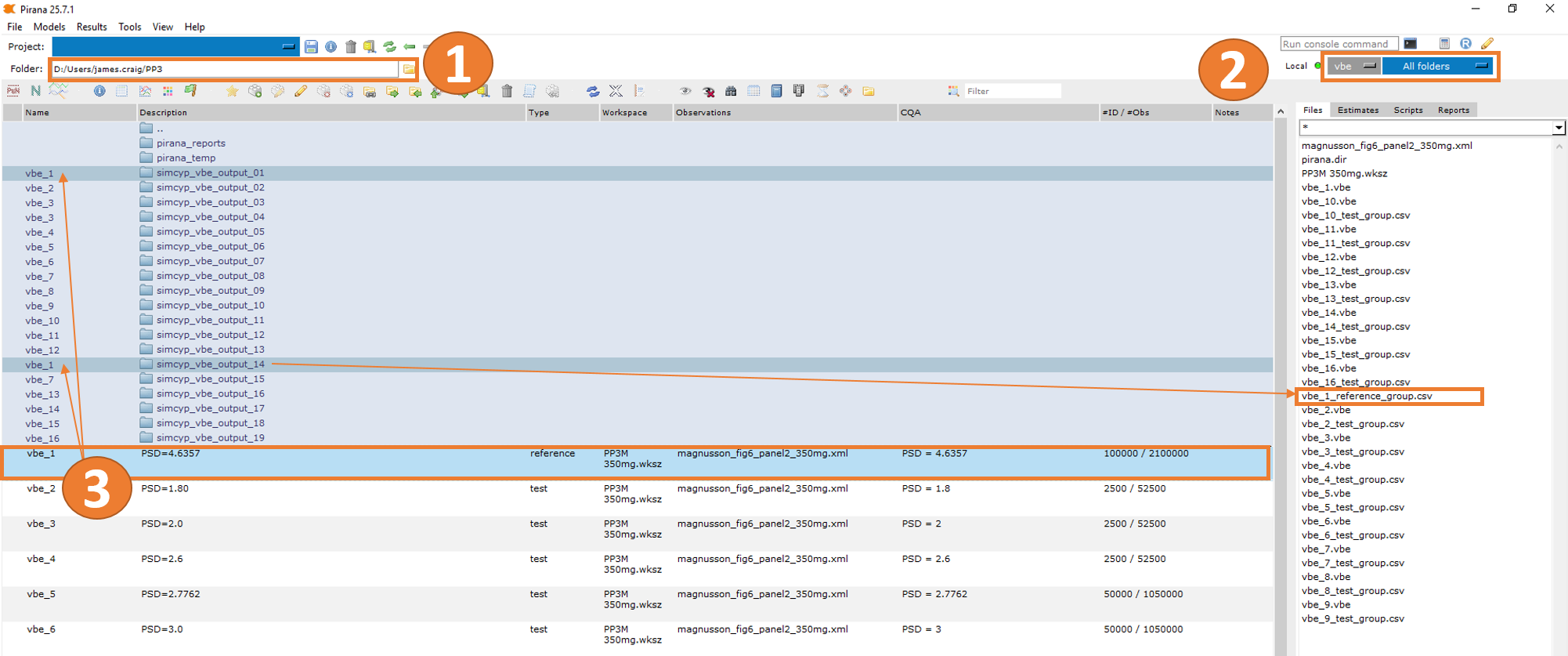
File Organization

When you select vbe_1 in the Pirana table, you’ll see that Simcyp^TM simulation output subfolders (e.g., simcyp_vbe_output_01 and simcyp_vbe_output_14) are “attached” to the VBE object (as illustrated in item 3 in the figure above).

These subfolders contain the simulation results from the Simcyp^TM simulations executed in the Shiny application. Each time a new Shiny session is launched and a simulation is run for the selected vbe, upon exiting the Shiny session, the most recent simulation file generated is automatically copied from the simulation output folder to the Pirana working directory and renamed to {vbe_name}_{vbe_type}_group.csv (e.g., vbe_1_reference_group.csv).

Note: To keep the example file size manageable, the simulation output subfolders contain only a subset of subjects from the full simulation runs. Complete simulation results with all subjects are available in the corresponding .csv files located in the Pirana working directory (e.g., vbe_1_reference_group.csv).

Phase 1: Reference Group Simulation (Optional)

Note: Since simulation results are pre-generated in the example files, you can skip Phases 1-3 and proceed directly to Phase 4: Statistical Analysis if you want to explore the R script functionality immediately.

Step 1: Create Reference VBE

1. Navigate to the top-level menu in Pirana
2. Select Models > New Model (or use the shortcut Ctrl + n)
3. This will launch the ‘Create VBE’ dialog

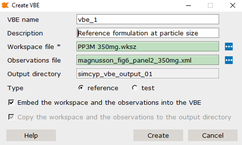
Step 2: Configure Reference VBE Settings

VBE Configuration

• VBE Name: vbe_1 (default)
• Description: “Paliperidone Palmitate Reference Formulation”
• Type: Reference

File Selection

• Workspace File: PP3M 350mg multidose June 24 variability calibrated model newseed.wksz
• Observations File: magnusson_fig6_panel2_350mg.xml

This workspace file contains calibrated input parameters for the reference group formulation with the Particle Size Distribution Mean Radius parameter value set to 4.6357.

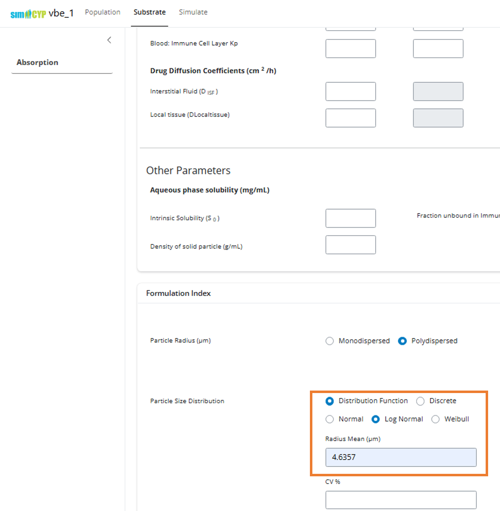
Step 3: Set Reference Parameters

1. Navigate to the Formulation Index section under Substrate > Absorption
2. Set the PSD Mean Radius parameter value to 4.6357

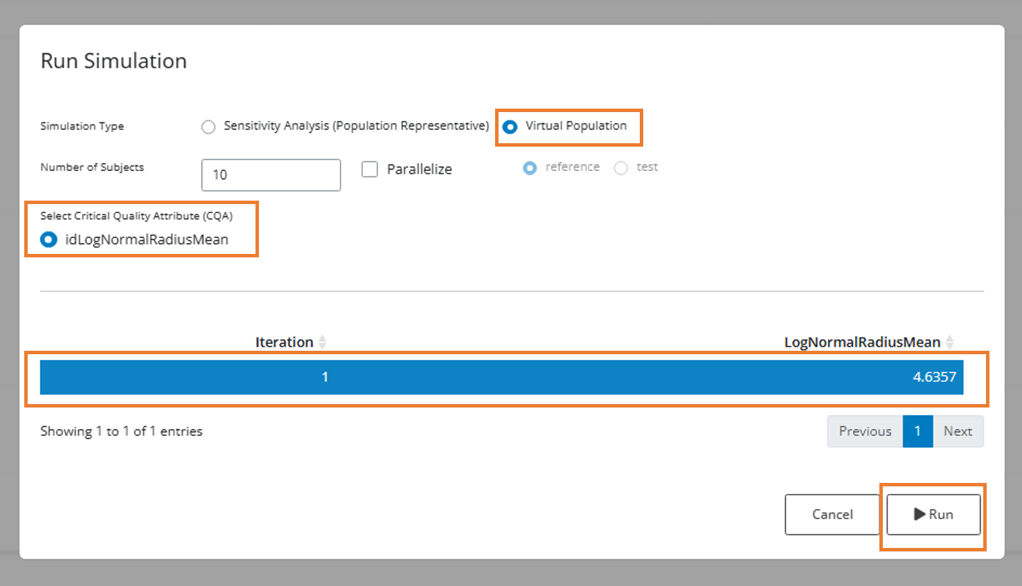
Step 4: Run Reference Simulation

1. Navigate to the Simulate tab in the top menu
2. Click the Simulate button in the left sidebar

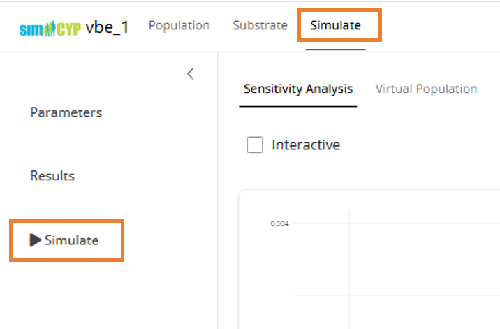
3. Configure the simulation settings:
   • Virtual Population: Select this radio button
   • Number of Subjects: 100,000
   • Parallelize: Check this box for faster simulation
   • Parameter Table: Select the row with PSD Mean Radius = 4.6357

Step 5: View Reference Results

After clicking ‘Run’, navigate to Results > Virtual Population to visualize your simulation results.

Phase 2: Sensitivity Analysis (Optional)

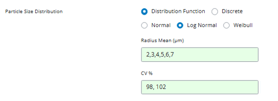
Step 1: Set Multiple Parameter Values

Return to the parameter input that you set for the reference group. For sensitivity analysis, you’ll want to test multiple PSD values around the reference value.

The application supports three input formats:

• Single value: 4.6357
• Comma-separated list: 1.8000, 2.0000, 2.6000, 2.7762, 3.0000, 4.6357, 4.8375, 5.0679, 5.5000, 6.2300, 6.4500, 6.7000, 7.1000, 7.5000
• Sequence statement: seq(1.8, 7.5, 0.5) (sequence from 1.8 to 7.5 by 0.5)

For this example, let’s test values around our reference value of 4.6357:

Step 2: Preview Parameter Combinations

Navigate to the Simulate tab and select Parameters. You’ll see an expanded grid showing all unique parameter combinations given the input values we’ve set:

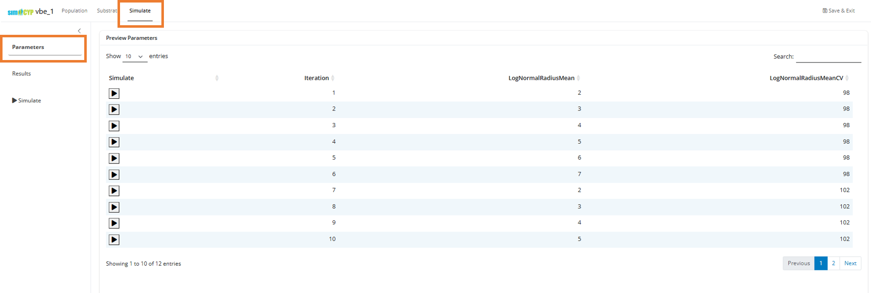
The iteration number corresponds to the unique identifier for each parameter combination.

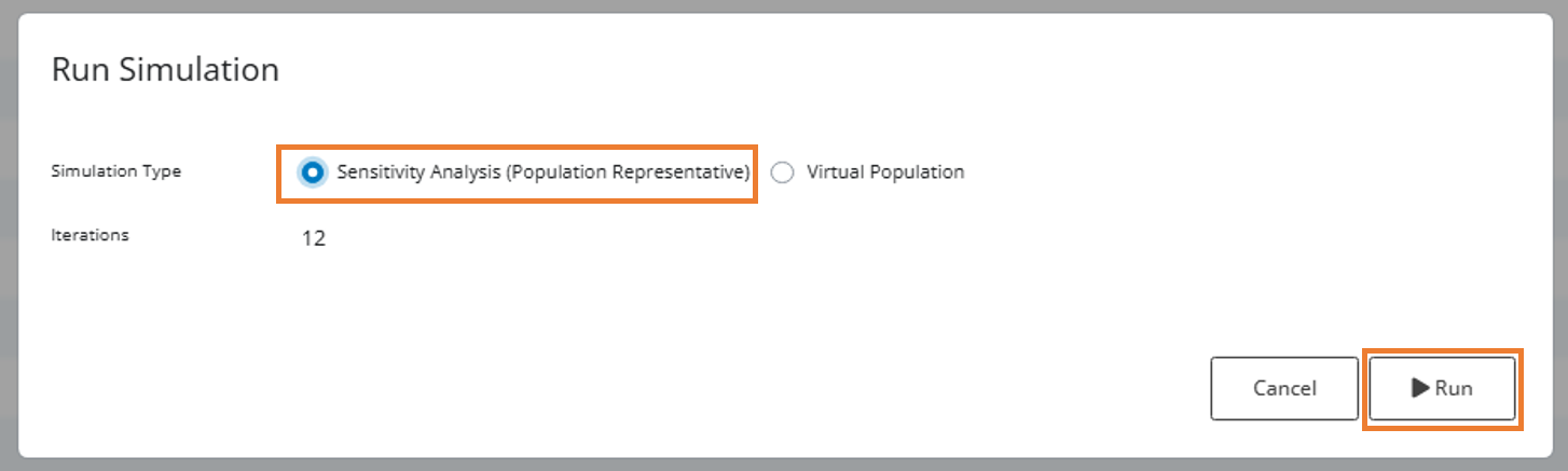
Step 3: Run Sensitivity Analysis

Instead of simulating individual parameter combinations, select the “Sensitivity Analysis (Population Representative)” radio button. This will perform simulations for a representative subject in the population for each unique parameter combination.

Step 4: Analyze Sensitivity Results

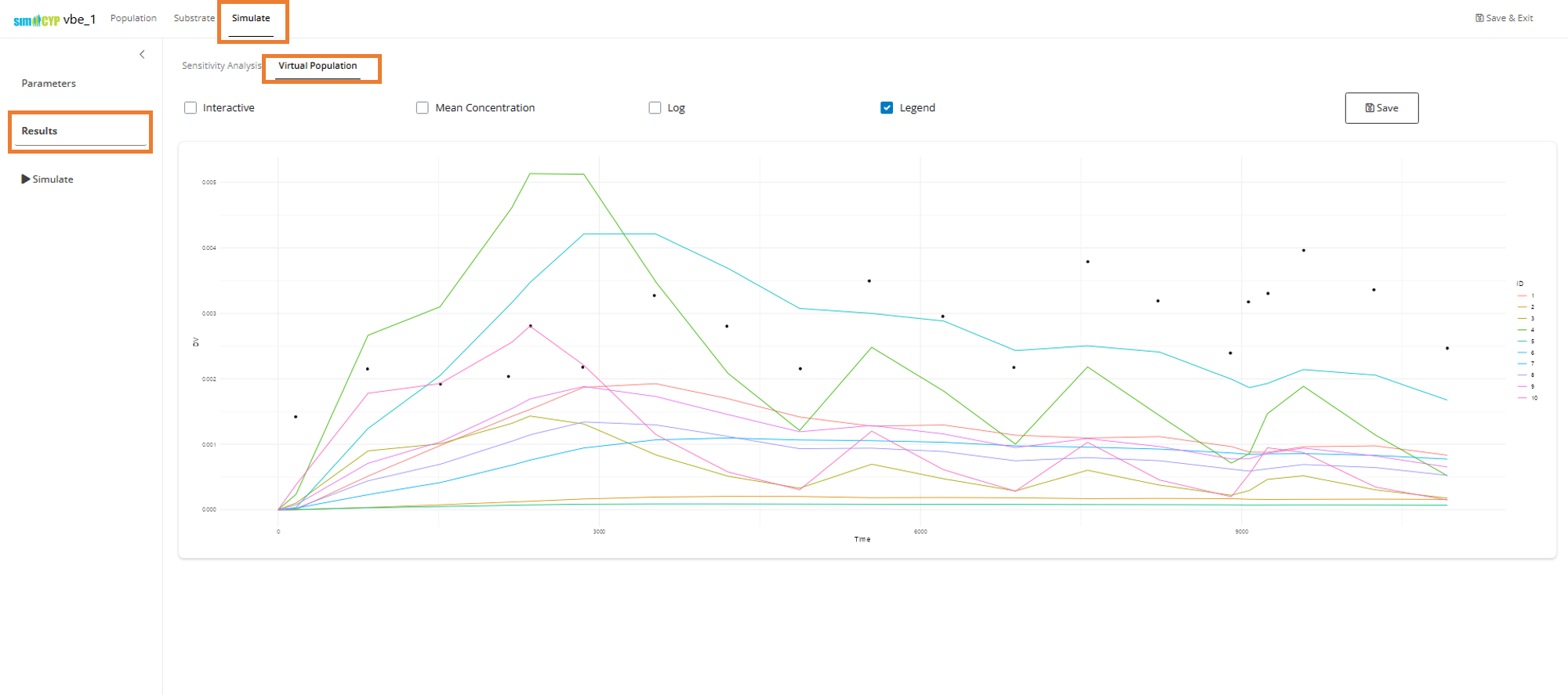
Navigate to the Results tab and select Sensitivity Analysis to view your sensitivity analysis results:

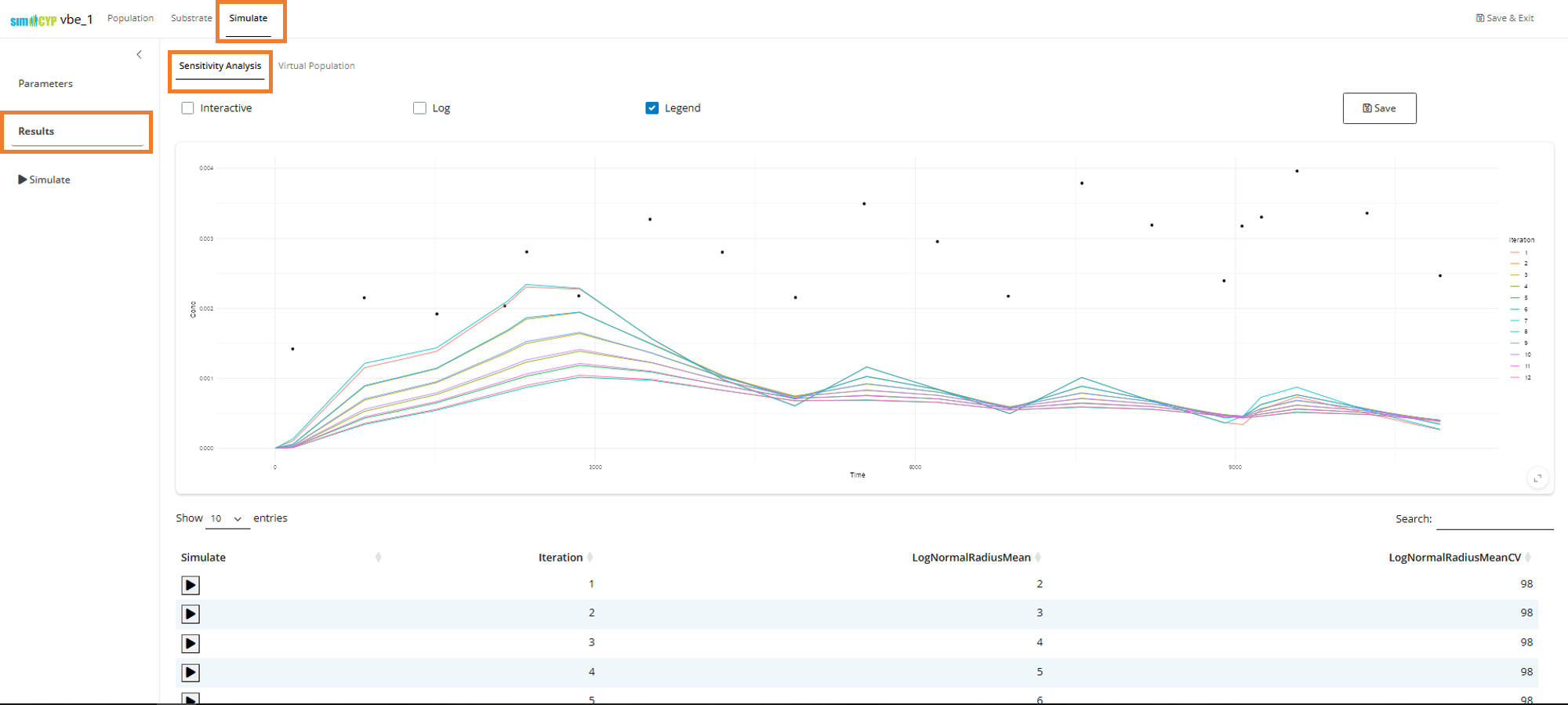
You can select any row in the table to observe the best fit through the data.

Note: Because the drug has very high variance and the distributions are log-normal, we’re seeing that the observed median value (points) is higher than the population representative predictions (lines) returned in the above sensitivity analysis plot.

Phase 3: Test Group Simulations (Optional)

Based on your sensitivity analysis, you can now identify the CQA values you want to test for bioequivalence. You will need to create a separate VBE for each test CQA value you want to evaluate.

This process is iterative. You don’t need to create all VBEs upfront. Instead, you typically:

1. Start with a single test CQA value and simulate a certain number of subjects
2. Run R scripts to compare test results against your reference
3. Check bioequivalence statistics
4. Adjust simulations as needed (increase subjects, modify parameters)
5. Repeat the process until you achieve the desired statistical power

Creating Test VBEs

For each test CQA value you want to evaluate:

1. Create a new VBE using the same steps as for the reference group (using the same .wksz)
2. In the Create VBE dialog, select the ‘test’ option instead of ‘reference’
3. Set the specific CQA value for this test formulation
4. Run the virtual population simulation with the appropriate number of subjects
5. Compare results with your reference group

Example Test VBE Creation

For the Paliperidone study, you would create separate VBEs for each PSD mean radius value:

• vbe_2: PSD Mean Radius = 1.8000 (2,500 subjects)
• vbe_3: PSD Mean Radius = 2.0000 (2,500 subjects)
• vbe_4: PSD Mean Radius = 2.6000 (2,500 subjects)
• … and so on for all test values

Phase 4: Statistical Analysis

Once you have completed simulations for both reference and test groups, you can perform comprehensive statistical analysis using the integrated R scripts in Pirana.

Available Analysis Scripts

The VBE R script library is located in the Pirana installation folder (e.g., {Pirana_Installation_Directory}/scripts/VBE). With the VBE context selection selected in Pirana, the scripts will automatically be visible in the scripts tab.

---

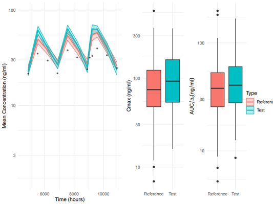
1. Compare Simulations

These scripts allow users to plot the time-concentration profiles with confidence intervals and additional plots for comparing AUC and CMax. Users can supply time filtering values to calculate AUC and CMax in a specific dosing region.

Comparison of mean concentration-time profiles between reference (PSD = 4.6357 µm) and test (PSD = 2.6 µm) formulations. The plot shows confidence intervals and highlights differences in bioavailability across user-specified time intervals. Generated by the compare_predictions.R script.

---

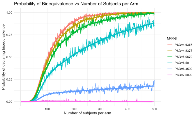
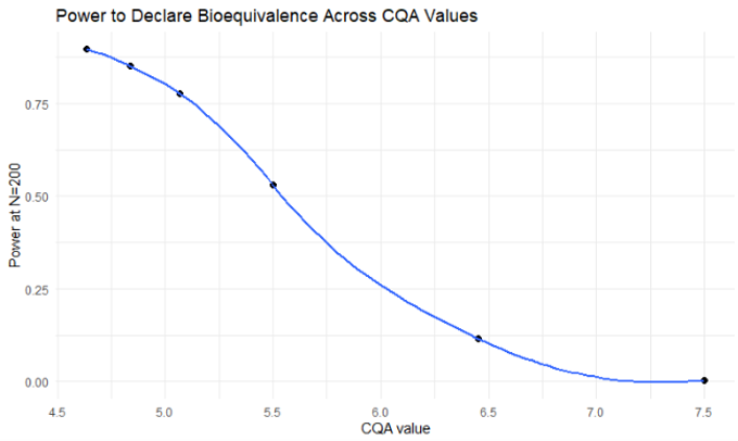
2. Power Curve vs Sample Size Analysis

This functionality estimates the statistical power (i.e., the probability of declaring bioequivalence) of TOST test assessments for VBE trials of varying sizes. A bootstrap Monte Carlo resampling algorithm is used to form VBE trials of different arm sizes from a large pool of simulated patients.

Output from calculate_subjects_per_arm.R script in Pirana, showing statistical power curves (probability of declaring bioequivalence) as a function of number of subjects per arm for different CQA values. Both raw and smoothed curves are presented

Output from calculate_power_trial_size.R script in Pirana, displaying the power to declare bioequivalence at a fixed trial size (e.g., N = 200) across varying CQA values.

---

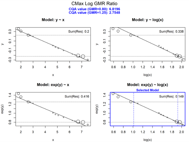
3. CQA Sensitivity Analysis

The cqa_sensitivity.R script evaluates the relationship between a CQA and the geometric mean ratio (GMR) of either Cmax or AUC in VBE simulations. It computes subject-level Cmax and AUC values from reference and test datasets, optionally adding log-normal noise derived from a user-defined sigma or estimated from observed data.

Model selection for assessing the sensitivity of Cmax Log GMR to the CQA, here represented as PSD mean radius. Four candidate models are evaluated (y ~ x, y ~ log(x), exp(y) ~ x, and exp(y) ~ log(x)) using weighted residuals. Circle sizes are scaled by GMR variance. The best-fitting model—exp(y) ~ log(x) in this example—is outlined in blue. Vertical dashed lines indicate the estimated CQA values corresponding to GMR thresholds of 0.80 and 1.25; CQA values provided in plot subtitle. This plot is generated by the cqa_sensitivity.R script integrated within Pirana.

---

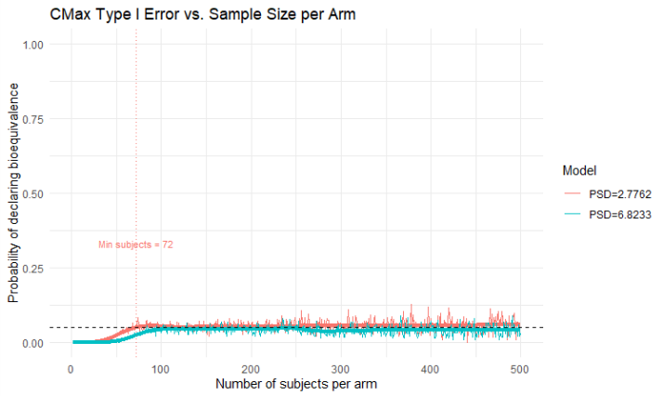
4. Type 1 Error Analysis

Estimates the type 1 error by calculating the probability of declaring bioequivalence for test drugs that are on the edge of the 0.8 - 1.25 GMR range.

Type 1 error rate versus number of subjects per arm, based on TOST assessments of Cmax. The dotted line indicates the 5% significance level. Both formulations shown (PSD mean radii of 2.7762 and 6.8233 µm) correctly maintain type 1 error around the pre-defined 5% level across increasing trial sizes. This plot is generated by the type_I_error.R script integrated within Pirana.

---

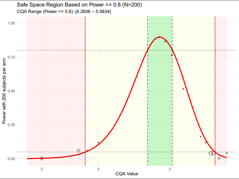
5. Safe Space Analysis

This script generates a plot of the safe space and will return the CQA bounds of this region to the user. Within this visualization, the region in which the population level GMRs are within the 0.8 to 1.25 range (as informed by the CQA sensitivity analysis) is highlighted to users.

Plot of safe space of test formulations bioequivalent to a reference. The overlaid curve shows the power to declare bioequivalence at a fixed trial size (e.g., 500 subjects per arm) across varying CQA values. Simulated points are scaled by variance to highlight precision, with larger points corresponding to larger variance. The green area represents the formulations with population level GMRs within the 0.8 – 1.25 BE region, while red regions indicate values outside those BE limits. The safe space region, within which power exceeds 80%, will be a fraction of the region highlighted in green in this plot. The CQA boundaries of the safe space are also returned to the user.

Running Statistical Analysis

1. Select your VBE objects in Pirana (reference and test VBEs, use ctrl/shift for multi-selection)
2. Navigate to the Scripts tab in Pirana
3. Choose the appropriate analysis script based on your objectives
4. Configure script parameters as needed
5. Execute the analysis and review results

Results and Interpretation

Key Findings

1. Power Analysis: A trial size of 200 subjects per arm was determined to provide 85% power for the 4.8 µm radius test case
2. Type I Error: The analysis correctly maintained type I error around the 5% level across increasing trial sizes
3. Safe Space: The analysis identified the safe space boundaries where test formulations maintain bioequivalence with adequate statistical power

Statistical Power

The power analysis revealed that: - Smaller trial sizes (e.g., 50 subjects per arm) provide insufficient power for most test formulations - Larger trial sizes (e.g., 200+ subjects per arm) provide adequate power for formulations within the bioequivalence region - The relationship between CQA values and power is non-linear, with power decreasing rapidly as formulations move away from the reference

Type I Error Control

The type I error analysis demonstrated that: - Formulations at the bioequivalence boundaries (GMR = 0.8 and 1.25) correctly maintain type I error around 5% - The statistical methodology properly controls for false positive declarations of bioequivalence - The analysis provides confidence in the robustness of the VBE approach

Safe Space Boundaries

The safe space analysis identified: - The range of PSD mean radius values that maintain bioequivalence - The region where statistical power exceeds 80% for a given trial size - Practical boundaries for formulation development and quality control

Conclusions

This Paliperidone Palmitate case study demonstrates the comprehensive capabilities of the Pirana-Simcyp^TM VBE workflow. The analysis successfully:

1. Established a robust reference simulation with 100,000 subjects
2. Performed systematic sensitivity analysis across multiple CQA values
3. Generated test simulations for multiple formulations
4. Conducted comprehensive statistical analysis including power, type I error, and safe space assessment
5. Provided actionable results for formulation development and quality control

The iterative nature of the VBE process allows researchers to refine their analysis based on preliminary results, making it a powerful tool for bioequivalence assessment in drug development.

Next Steps

After completing this analysis, you can:

• Compare reference and test group results

• Perform additional statistical analysis for bioequivalence assessment

• Generate reports and visualizations

• Share your complete VBE project files

Acknowledgements

This package was developed with support from the U.S. Food and Drug Administration (FDA) through the grant 1U01FD007904-01, titled “A State-of-the-Art Virtual Bioequivalence Platform and Case Studies on Complex Formulations, Systemic and Local Concentration-based Bioequivalence”.